中文 | English

Transforming Linear Regression into a Neural Network

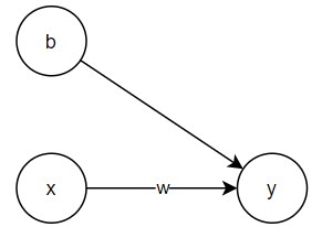
Linear regression can also be viewed as a simple neural network. Consider a univariate linear regression model with one feature:

$$ \begin{aligned} y = w \cdot x + b \end{aligned} $$

This can be represented in the following neural network structure:

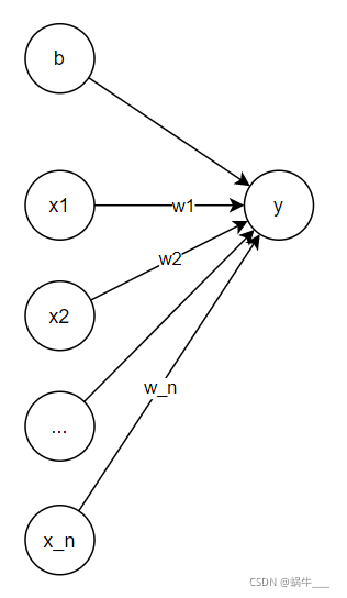
If we generalize $x$ into a vector, i.e., $x=(x_1, x_2, ... , x_n)$, the corresponding neural network structure becomes:

Implementing Univariate Linear Regression with PyTorch

Code Implementation for Univariate Linear Regression Using PyTorch

```python
import torch
import matplotlib.pyplot as plt
```

First, generate test data:

```python
X = torch.rand(100, 1) * 10  # Generates 100 rows with one column, uniformly distributed in [0,10]
X[:3]
```

```
tensor([[3.7992],
        [5.5769],
        [8.8396]])
```

```python
y = 3 * X + 10 + torch.randn(100, 1) * 3 # Calculate corresponding y values; y is also 100 rows by 1 column
y[:3]
```

```
tensor([[19.4206],
        [29.7004],
        [38.3561]])
```

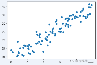
Next, plot the data to visualize it:

```python
plt.scatter(X.numpy(), y.numpy())
plt.show()
```

Now, define the linear regression model:

```python
class LinearRegression(torch.nn.Module):
    """
    The model inherits `torch.nn.Module`, a required superclass for models in PyTorch.
    """

    def __init__(self):
        super().__init__()  # Initialize the base class

        """
        Define the first layer (linear layer) of the neural network. Important parameters:
        in_features: Number of input neurons
        out_features: Number of output neurons
        bias: Whether to include a bias term

        For more on torch.nn.Linear, refer to: https://pytorch.org/docs/stable/nn.html#linear-layers
        """
        self.linear = torch.nn.Linear(in_features=1, out_features=1, bias=True)

    def forward(self, x):
        """
        Forward propagation to compute the network’s output
        """
        predict = self.linear(x)
        return predict    
```

With this, the model is defined. Now, initialize the model:

```python
model = LinearRegression() # Initialize model
```

Define the optimizer, choosing stochastic gradient descent:

```python
"""
torch.optim.SGD accepts key parameters:

- params: Model parameters
- lr: Learning rate
"""
optimizer = torch.optim.SGD(model.parameters(), lr=1e-3)

# View model parameters
for param in model.parameters():  # model.parameters returns an iterable object for multiple parameters
    print(param)
```

```
Parameter containing:
tensor([[-0.0462]], requires_grad=True)
Parameter containing:
tensor([-0.5942], requires_grad=True)
```

Define the loss function, here using MSE (mean squared error):

```python
loss_function = torch.nn.MSELoss()
```

Now we can start training the model:

```python
for epoch in range(10000): # Train for 10,000 epochs
    """
    1. Pass X through the model to compute predicted y values
    X.shape and predict_y.shape are both (100,1)
    """
    predict_y = model(X) 

    """
    2. Calculate loss using the loss function
    """
    loss = loss_function(predict_y, y)

    """
    3. Perform backpropagation
    """
    loss.backward()

    """
    4. Update weights
    """
    optimizer.step()

    """
    5.Clear the optimizer’s gradient to avoid interference in the next iteration
    """
    optimizer.zero_grad()
```

Finally, view the final parameters to verify the result:

```python
for param in model.parameters(): # model.parameters returns an iterable object for multiple parameters
    print(param)
```

```
Parameter containing:
tensor([[3.0524]], requires_grad=True)
Parameter containing:
tensor([9.2819], requires_grad=True)
```

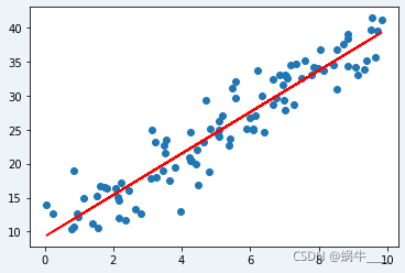
Let's plot the final result:

```python
plt.scatter(X, y)
plt.plot(X, model(X).detach().numpy(), color='red')
plt.show()
```