中文 | English

Blog Content

In this article, we’ll implement a handwritten digit recognition model for the MNIST dataset using a basic BP (backpropagation) neural network. Let's dive right in.

Import Required Packages

```python
import os
import numpy as np
import torch
import torchvision
import matplotlib.pyplot as plt
from time import time
from torchvision import datasets, transforms
from torch import nn, optim
```

Set Up Transformations

We define a transform object to standardize the images in the dataset:

```python
transform = transforms.Compose([transforms.ToTensor(),
                                transforms.Normalize((0.5,), (0.5,)),])
```

Load Training Data

We’ll load and, if necessary, download the training dataset using PyTorch’s API:

```python
train_set = datasets.MNIST('train_set',  # save here
                          download=not os.path.exists('train_set'), # download if not exists
                          train=True, # use training set
                          transform=transform # apply transform
                         )
train_set
```

```
Dataset MNIST
    Number of datapoints: 60000
    Root location: train_set
    Split: Train
    StandardTransform
Transform: Compose(
               ToTensor()
               Normalize(mean=(0.5,), std=(0.5,))
           )
```

After downloading, we’ll see the training set contains 60,000 images. Next, we download the test dataset:

```python
test_set = datasets.MNIST('test_set', 
                        download=not os.path.exists('test_set'),
                        train=False, 
                        transform=transform
                       )
test_set
```

```
Dataset MNIST
    Number of datapoints: 10000
    Root location: test_set
    Split: Test
    StandardTransform
Transform: Compose(
               ToTensor()
               Normalize(mean=(0.5,), std=(0.5,))
           )
```

The test dataset has 10,000 images.

Create Data Loaders

Next, we’ll use DataLoader to manage batching for both training and testing datasets:

```python
train_loader = torch.utils.data.DataLoader(train_set, batch_size=64, shuffle=True)
test_loader = torch.utils.data.DataLoader(test_set, batch_size=64, shuffle=True)

dataiter = iter(train_loader)
images, labels = dataiter.next()

print(images.shape)
print(labels.shape)
```

```
torch.Size([64, 1, 28, 28])
torch.Size([64])
```

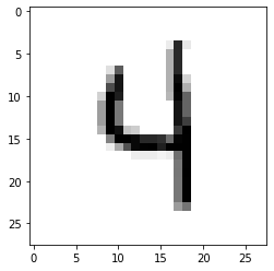
The output shows that each batch contains 64 grayscale images, each sized 28x28 pixels. Let’s display one image:

```python
plt.imshow(images[0].numpy().squeeze(), cmap='gray_r');
```

With this, our initial setup is done.

Define the Neural Network

```python
class NeuralNetwork(nn.Module):

    def __init__(self):
        super().__init__()

        """
        Define the first linear layer:
        Input: image (28x28 pixels)
        Output: input to the first hidden layer with 128 units
        """
        self.linear1 = nn.Linear(28 * 28, 128)
        # Apply ReLU activation in the first hidden layer
        self.relu1 = nn.ReLU()

        """
        Define the second linear layer:
        Input: output from the first hidden layer
        Output: input to the second hidden layer with 64 units
        """
        self.linear2 = nn.Linear(128, 64)
        # Apply ReLU activation in the second hidden layer
        self.relu2 = nn.ReLU()

        """
        Define the third linear layer:
        Input: output from the second hidden layer
        Output: output layer with 10 units
        """
        self.linear3 = nn.Linear(64, 10)
        # Apply softmax for normalization at the output layer
        self.softmax = nn.LogSoftmax(dim=1)

        # Alternatively, define the model using nn.Sequential:
        self.model = nn.Sequential(
            nn.Linear(28 * 28, 128),
            nn.ReLU(),
            nn.Linear(128, 64),
            nn.ReLU(),
            nn.Linear(64, 10),
            nn.LogSoftmax(dim=1)
        )

    def forward(self, x):
        """
        Define the forward pass of the neural network
        x: image data with shape (64, 1, 28, 28)
        """
        # Reshape x to (64, 784)
        x = x.view(x.shape[0], -1)

        # Forward propagation
        x = self.linear1(x)
        x = self.relu1(x)
        x = self.linear2(x)
        x = self.relu2(x)
        x = self.linear3(x)
        x = self.softmax(x)

        # Alternatively, this could be done using x = self.model(x)

        return x
```

```python
model = NerualNetwork()
```

After defining the neural network, we set up the loss function, using Negative Log Likelihood Loss (NLLLoss), which is common for classification tasks.

```python
criterion = nn.NLLLoss()
```

Then, we define the optimizer, using Stochastic Gradient Descent with a learning rate of 0.003 and the default momentum of 0.9 (to reduce overfitting).

```python
optimizer = optim.SGD(model.parameters(), lr=0.003, momentum=0.9)
```

With the setup complete, we start training the dataset:

```python
time0 = time() # Record the start time
epochs = 15  # Train for 15 epochs
for e in range(epochs):
    running_loss = 0  # Initialize the loss for the epoch
    for images, labels in train_loader:
        # Forward pass to get predictions
        output = model(images) 

        # Compute the loss
        loss = criterion(output, labels) 

        # Backward pass
        loss.backward()

        # Update weights
        optimizer.step()

        # Clear gradients
        optimizer.zero_grad() 

        # Accumulate the loss
        running_loss += loss.item()
    else:
        # Print the loss after each epoch
        print("Epoch {} - Training loss: {}".format(e, running_loss/len(train_loader)))

# Print total training time
print("\nTraining Time (in minutes) =",(time()-time0)/60)
```

```
Epoch 0 - Training loss: 0.6462286284117937
Epoch 1 - Training loss: 0.27847810615418056
...
Epoch 13 - Training loss: 0.056689855163551565
Epoch 14 - Training loss: 0.05361823974547586

Training Time (in minutes) = 2.9436919848124186
```

On my machine, the training took just over 2 minutes to complete, with the loss decreasing steadily.

Next, we’ll evaluate the model:

```python
correct_count, all_count = 0, 0
model.eval() # Set the model to evaluation mode

# Load images batch by batch from the test_loader
for images,labels in test_loader:
    # Loop through the batch to evaluate each image
    for i in range(len(labels)):
        logps = model(images[i])  # Forward pass to get predictions
        probab = list(logps.detach().numpy()[0]) # Convert prediction to a list of probabilities
        pred_label = probab.index(max(probab)) # Get the index of the highest probability as the predicted label
        true_label = labels.numpy()[i]
        if(true_label == pred_label): # Check if the prediction is correct
            correct_count += 1
        all_count += 1

print("Number Of Images Tested =", all_count)
print("Model Accuracy =", (correct_count/all_count))
```

```
Number Of Images Tested = 10000
Model Accuracy = 0.9741
```

The model achieved an accuracy of 97.41% on the test dataset.

---

References

Handwritten Digit Recognition Using PyTorch — Intro To Neural Networks： https://towardsdatascience.com/handwritten-digit-mnist-pytorch-977b5338e627