Intuitive Guide for Temperature Coefficients in Contrastive Learning
Table of Content
1. Overview of Contrastive Learning
If you haven't studied contrastive learning before, it's highly recommended to do so. This section only serves as a review.
Purpose of Contrastive Learning:The primary goal of contrastive learning is to bring similar samples closer together in the feature space while pushing dissimilar samples further apart. This encourages a more evenly distributed feature representation in the space.
Key Steps in Contrastive Learning:
- Construct positive and negative pairs:
- Positive pair: $(x_i, x_j)$, where $x_i$ and $x_j$ are similar samples (e.g., two images of dogs).
- Negative pair: $(x_i, y_j)$, where $x_i$ and $y_j$ are dissimilar samples (e.g., an image of a dog and an image of a cat).
- Measure similarity: To achieve the desired distribution, a similarity function (typically cosine similarity) is used:
- $\text{sim}(x_i, x_j)$ should be as large as possible for positive pairs.
- $\text{sim}(x_i, y_j)$ should be as small as possible for negative pairs.
Here, $x_i$ is referred to as the anchor, $x_j$ as the positive sample, and $y_j$ as the negative sample.
Loss Function in Contrastive Learning:Contrastive learning uses a loss function similar to the Cross-Entropy Loss employed in multi-class classification tasks.
Why Cross-Entropy Loss Works?
Let’s first recall how multi-class classification works. Assume we have 4 classes: $[c_1, c_2, c_3, c_4]$. The output probabilities are represented as $y = [y_1, y_2, y_3, y_4]$. If the sample belongs to class $c_1$, we want $y_1$ to be as large as possible while minimizing $y_2, y_3, y_4$.
In contrastive learning, consider 1 positive sample $(x'_1)$ and 3 negative samples $(y_2, y_3, y_4)$. By computing the similarity scores between $x$ and these samples, we get $[\text{sim}(x, x'_1), \text{sim}(x, y_2), \text{sim}(x, y_3), \text{sim}(x, y_4)]$. The goal is similar: maximize $\text{sim}(x, x'_1)$ while minimizing the other similarity scores.
Thus, Cross-Entropy Loss is a natural fit for contrastive learning. The loss function is typically expressed as:
$$ \begin{aligned} L_c = - \log \frac{\exp \left(\operatorname{sim}\left(x, x'_i\right) / \tau\right)}{\sum_{j=1}^n \exp \left(\operatorname{sim}\left(x, y_j\right) / \tau\right)} \end{aligned} $$
Here, $\tau$ is a temperature scaling factor that adjusts the sharpness of the distribution.
Note: While the exact formula may vary slightly across papers, the core idea remains consistent.
2. Intuitively Understanding Contrastive Learning
To better understand the impact of contrastive learning, let’s walk through an example using the following code.
First, we start by importing the necessary libraries:
```python
import matplotlib.pyplot as plt
import torch
from torch import nn
import random
import numpy as np
import torch.nn.functional as F
from tqdm import tqdm
import copy
```
Next, we define two utility classes:
```python
def setup_seed(seed):
    torch.manual_seed(seed)
    torch.cuda.manual_seed_all(seed)
    np.random.seed(seed)
    random.seed(seed)
    torch.backends.cudnn.deterministic = True

def plot_samples(samples, labels):
    plt.xlim(-1.1, 1.1)
    plt.ylim(-1.1, 1.1)

    plt.scatter(samples[labels==0, 0], samples[labels==0, 1], color='blue')
    plt.scatter(samples[labels==1, 0], samples[labels==1, 1], color='yellow')
    plt.scatter(samples[labels==2, 0], samples[labels==2, 1], color='black')
    plt.scatter(samples[labels==3, 0], samples[labels==3, 1], color='red')

    # draw the x-axis
    plt.annotate("", xy=(1, 0), xycoords='data', xytext=(-1, 0), textcoords='data',
                 arrowprops=dict(arrowstyle="->", connectionstyle="arc3"))
    # draw the y-axis
    plt.annotate("", xy=(0, 1), xycoords='data', xytext=(0, -1), textcoords='data',
                 arrowprops=dict(arrowstyle="->", connectionstyle="arc3"))
    plt.show()

setup_seed(0)
```
Let’s begin the demonstration by defining 100 samples. Each sample has two features (x, y), and labels range from (0, 1, 2, 4), representing the quadrant they belong to:
```python
samples = torch.rand(100, 2)
samples[25:50, 0] -= 1
samples[50:75, :] -= 1
samples[75:100, 1] -= 1
labels = torch.LongTensor([0] * 25 + [1] * 25 + [2] * 25 + [3] * 25)
```
We then plot the samples, as shown below:
```python
plot_samples(samples, labels)
```
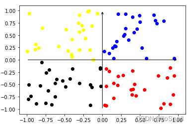
Afterward, we define an encoder to simulate the role of feature extractors such as convolutional networks or BERT:
```python
encoder = nn.Sequential(
    nn.Linear(2, 10, bias=False),
    nn.Linear(10, 2, bias=False),
    nn.Tanh()
)
```
Once the samples are passed through the encoder, the extracted features are plotted in the following diagram:
```python
plot_samples(encoder(samples).clone().detach(), labels)
```
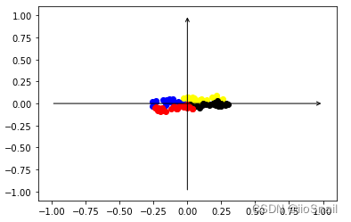
From the diagram, we can observe that the features extracted by the encoder are densely clustered together. This tight clustering makes it challenging for downstream networks to classify them effectively.
This is where contrastive learning comes into play. The goal of contrastive learning is to make similar samples closer to each other and push dissimilar ones further apart. This results in a more evenly distributed feature space, which improves classification performance.
Note: This example is not perfect because the similar samples are already quite close to one another.
Finally, let’s prepare the code to train the encoder using contrastive learning:
```python
def train_and_plot(step=10000, temperature=0.05):
    """
    Arguments:
    step: Number of training iterations.
    temperature: A scaling factor that controls the sharpness of the similarity scores.
    """
    # Clone the encoder to ensure the original encoder remains unchanged
    encoder_ = copy.deepcopy(encoder)
    loss_fnt = nn.CrossEntropyLoss()
    optimizer = torch.optim.SGD(encoder_.parameters(), lr=3e-4)

    # Training loop with a batch size of 1 for simplicity
    for _ in tqdm(range(step)):
        # Randomly pick one of the 4 labels as the anchor's label
        anchor_label = random.randint(0, 3)

        # Select one sample as the anchor and another as the positive sample from the same class
        anchor_sample = samples[labels == anchor_label][random.sample(range(25), 1)]
        positive_sample = samples[labels == anchor_label][random.sample(range(25), 1)]

        # Select 3 negative samples from other classes
        negative_samples = samples[labels != anchor_label][random.sample(range(75), 3)]

        # Extract features for all samples using the encoder
        anchor_feature = encoder_(anchor_sample)
        positive_feature = encoder_(positive_sample)
        negative_feature = encoder_(negative_samples)

        # Compute similarity between anchor and both positive and negative samples
        positive_sim = F.cosine_similarity(anchor_feature, positive_feature)
        negative_sim = F.cosine_similarity(anchor_feature, negative_feature)

        # Concatenate similarities and scale them by the temperature parameter
        sims = torch.concat([positive_sim, negative_sim]) / temperature

        # Construct the label for CrossEntropyLoss. Since the positive sample is at index 0, the label is 0.
        sims_label = torch.LongTensor([0])

        # Calculate the loss
        loss = loss_fnt(sims.unsqueeze(0), sims_label.view(-1))
        loss.backward()

        # Update parameters
        optimizer.step()
        optimizer.zero_grad()

    # Visualize the results after training
    plot_samples(encoder_(samples).clone().detach(), labels)
```
Next, we can train the encoder with a temperature parameter of 0.05. After training, we can plot the feature vectors of the samples to observe the effect:
```python
train_and_plot(10000, temperature=0.05)
```
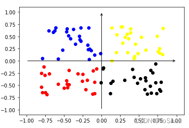
After applying contrastive learning, you can see that the feature distribution becomes more uniform and well-separated across different classes. This demonstrates the effectiveness of contrastive learning in producing better representations.
3. Comparing Different Temperature Coefficients in Contrastive Learning
In the previous section, we implemented a training function for contrastive learning. With this function, we can easily compare results by adjusting different parameters:
```python
train_and_plot(10000, temperature=0.99)
train_and_plot(10000, temperature=0.5)
train_and_plot(10000, temperature=0.05)
train_and_plot(10000, temperature=0.01)
train_and_plot(10000, temperature=0.001)
```
Here’s a visualization of the final results:
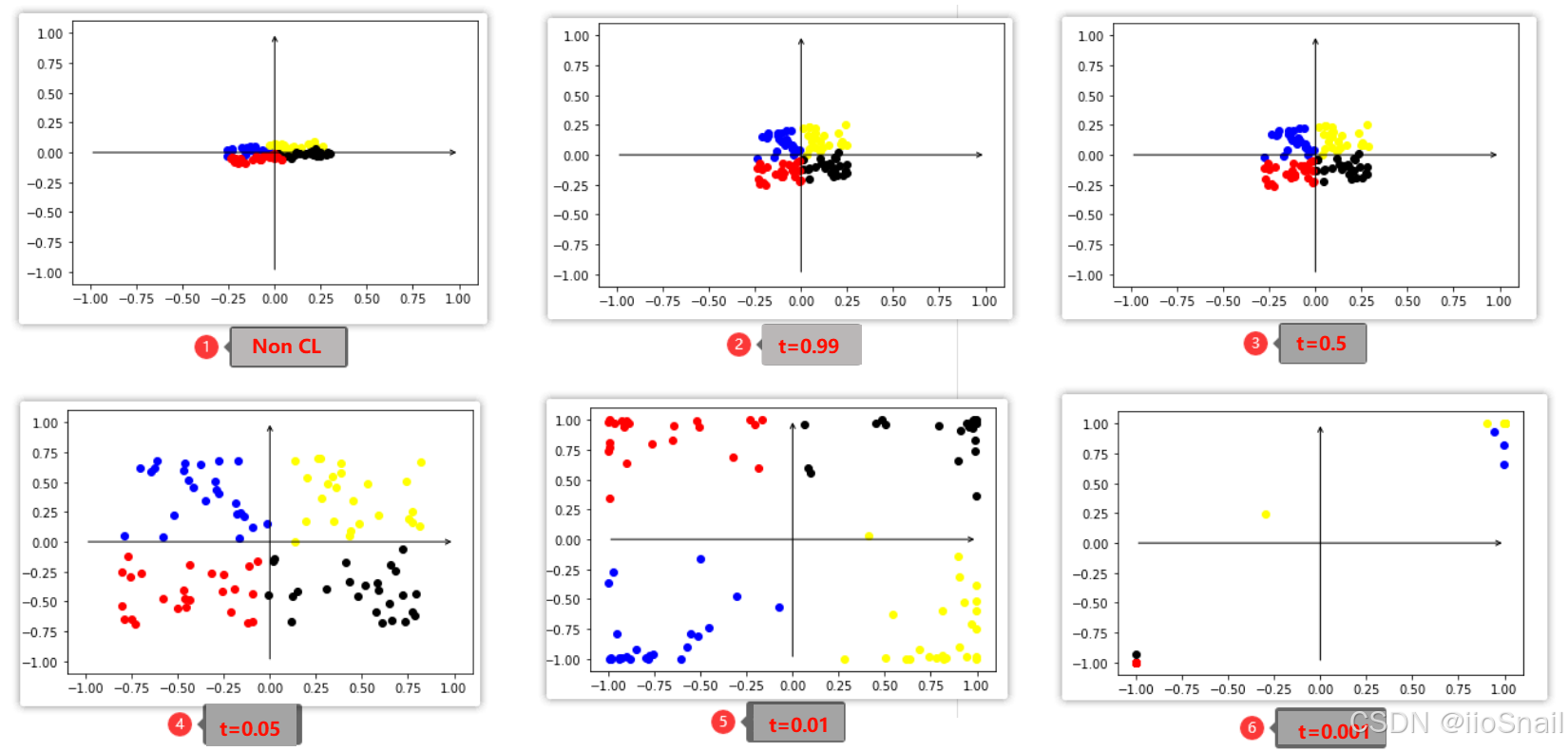
The sparse data points at the 0.001 temperature coefficient are seemingly vanishing or going out of bounds. In fact, this is caused by the Tanh activation function, which constrains the features to the range of (-1, 1). As a result, most points are concentrated at $(-1, 1)$ and $(-1, -1)$.
From the above visualization, we can draw the following conclusions:
- Smaller temperature coefficients improve contrastive learning performance. Specifically, similar samples are pulled closer together, while dissimilar samples are pushed further apart.
- To achieve a balanced and uniform feature distribution, the temperature coefficient needs to be moderate—values that are too high or too low can both be detrimental.
4. Analysis of Contrastive Learning Results
The above observations can be explained by analyzing how the loss function evolves with different temperature coefficients.
Let’s assume the similarity scores between an anchor sample and its positive/negative samples are as follows:
$[\text{sim}(x, x'_1), \text{sim}(x, y_2), \text{sim}(x, y_3), \text{sim}(x, y_4)]$ = [0.5, 0.25, -0.45, -0.1]
We can examine how the similarity values, Softmax probability distribution, and CrossEntropyLoss change as the temperature coefficient varies:
| Temperature | Similarity (sim) | Softmax Probabilities | CrossEntropyLoss |
|---|---|---|---|
| 1 | [0.5, 0.25, -0.45, -0.1] | [0.3684, 0.2869, 0.1425, 0.2022] | 0.9986 |
| 0.5 | [ 1.0, 0.5, -0.9, -0.2] | [0.4861, 0.2948, 0.0727, 0.1464] | 0.7214 |
| 0.05 | [10, 5, -9, -2] | [0.9933, 6.6e-03, 5.5e-09, 6.1-06] | 0.0067 |
| 0.01 | [ 50, 25, -45, -10] | [1.00, 1.3e-11, 5.5-42, 8.7-27] | 0 |
You can experiment with the table above using the following code snippet:
```python
t = 1   # Temperature
sims = torch.tensor([0.5, 0.25, -0.45, -0.1]) / t
print(sims)
prob = F.softmax(sims, dim=-1)
print(prob)
loss = F.cross_entropy(sims.unsqueeze(0), torch.LongTensor([0]))
print(loss)
```
Based on the table, we can derive the following conclusions:
(1) Lower temperature coefficients make the probability distribution sharper. This result is often visualized in other contrastive learning article as the following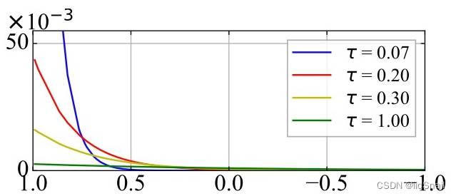
To better illustrate, we can use a Gaussian distribution representation:
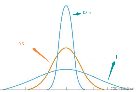
Note: These figures are illustrative and not rigorous; they are intended to demonstrate how temperature affects probability distribution.)
(2) When the anchor has the highest similarity with its positive sample, a lower temperature results in a lower loss.
Now, let’s analyze a scenario where the anchor sample has higher similarity with a negative sample. Suppose the similarity scores are:
$[\text{sim}(x, x'_1), \text{sim}(x, y_2), \text{sim}(x, y_3), \text{sim}(x, y_4)]$ = [0.25, 0.5, -0.45, -0.1]
The resulting changes in similarity, Softmax probabilities, and CrossEntropyLoss are as follows:
| Temperature | Similarity (sim) | Softmax Probabilities | CrossEntropyLoss |
|---|---|---|---|
| 1 | [0.25, 0.5, -0.45, -0.1] | [0.2869, 0.3684, 0.1425, 0.2022] | 1.2486 |
| 0.5 | [ 0.5, 1.0, -0.9, -0.2] | [0.2948, 0.4861, 0.0727, 0.1464] | 1.2214 |
| 0.05 | [5, 10, -9, -2] | [ 6.6e-03, 0.9933, 5.5e-09, 6.1-06] | 5.0067 |
| 0.01 | [ 25, 50, -45, -10] | [1.3e-11, 1.00, 5.5-42, 8.7-27] | 25 |
From these results, we can observe the relationship between temperature coefficients and loss:
- When the anchor sample has the highest similarity with the positive sample, a lower temperature leads to a lower loss.
- Conversely, when the anchor sample has the highest similarity with a negative sample, a lower temperature results in a significantly higher loss.
- Higher temperature coefficients result in a more moderate adjustment during training. The model is less sensitive to whether it correctly identifies the positive sample and makes smoother updates.
- Lower temperature coefficients cause sharper adjustments. The model prioritizes quickly learning to predict the positive sample correctly, and once it achieves this, further updates are minimal.
5. Final Thoughts on Temperature Coefficients
The conclusions presented here are based on my personal experiments and understanding. If there are any inaccuracies, please feel free to provide corrections or feedback in the comments.
Key takeaways regarding temperature coefficients in contrastive learning:
- Smaller temperature coefficients improve contrastive learning performance by pulling similar samples closer and pushing dissimilar samples further apart.
- To achieve uniform feature distribution, the temperature coefficient should be moderate—neither too high nor too low.
- When the anchor has the highest similarity with the positive sample, a lower temperature results in a lower loss.
- When the anchor has the highest similarity with a negative sample, a lower temperature significantly increases the loss.
- Higher temperature coefficients result in smoother and more moderate adjustments.
- Lower temperature coefficients lead to sharper, more aggressive adjustments, prioritizing the correct prediction of positive samples. Once learned, the model makes almost no further updates.
For points 1 and 2, refer to Section 3. For points 3–6, refer to Section 4.
The commonly used temperature coefficient is 0.05.


