图解通俗理解对比学习(Contrastive Learning)中的温度系数(temperature)

1. 对比学习简述
没有学过对比学习的,请学一下,这里只是复习。
对比学习目的:让相似的样本在空间中距离近一点,让不相似的样本距离远一点。这样就可以让特征分布在空间中更加均匀。
对比学习方法:
- 构建一个正样本对儿 $(x_i, x_j)$ ,和负样本对儿 $(x_i, y_j)$ ,其中$x_i$和$x_j$为相似的样本(例如两张狗的图片),而$x_i$和$y_j$为不相似的样本(例如狗和猫的图片)。
- 为了让相似的样本在空间中距离更近,不相似的样本在空间中更远,可以使用相似度函数(通常使用余弦相似度(cosine similarity))计算的相似度,即 $\text{sim}(x_i, x_j)$越大越好,$\text{sim}(x_i, y_j)$ 越小越好
这里的 $x_i$ 称为锚点,$x_j$ 称为正样本,$y_j$称为负样本
对比学习的Loss:
- 对比学习的Loss和多分类是一样的,都是使用的CrossEntropyLoss。
为什么使用CrossEntropyLoss可行呢,我们不妨来想一下多分类是怎么做的。
在多分类中,假设我们有4个类别,$[c_1, c_2, c_3, c_4]$,假设我们的输出为 $y = [y_1, y_2, y_3, y_4]$,若当前样本为$c_1$类别,那么我们则是希望 $y_1$ 越大越好,$y_2,y_3,y_4$越小越好。
在对比学习中,假设我们有1个正样本 $(x'_1)$,3个负样本 $(y_2, y_3, y_4)$,那么使用样本 $x$ 与它们计算的样本相似度为 $[\text{sim}(x, x'_1), \text{sim}(x, y_2), \text{sim}(x, y_3), \text{sim}(x, y_4)]$,此时我们同样是想让 $\text{sim}(x, x'_1)$ 越大越好,其他的越小越好呢。
所以,对比学习也使用CrossEntropyLoss。对比学习损失函数写作:
$$ \begin{aligned} L_c = - \log \frac{\exp \left(\operatorname{sim}\left(x, x'_i\right) / \tau\right)}{\sum_{j=1}^n \exp \left(\operatorname{sim}\left(x, y_j\right) / \tau\right)} \end{aligned} $$
虽然每个论文的公式写不太一样,但表达的意思都是一样的。
2. 直观感受下对比学习
为了感受对比学习的作用,我们将使用如下代码进行演示。
首先导入需要用到的包:
```python
import matplotlib.pyplot as plt
import torch
from torch import nn
import random
import numpy as np
import torch.nn.functional as F
from tqdm import tqdm
import copy
```
定义一些两个工具类:
```python
def setup_seed(seed):
    torch.manual_seed(seed)
    torch.cuda.manual_seed_all(seed)
    np.random.seed(seed)
    random.seed(seed)
    torch.backends.cudnn.deterministic = True

"""用于绘制样本"""
def plot_samples(samples, labels):
    plt.xlim(-1.1, 1.1)
    plt.ylim(-1.1, 1.1)

    plt.scatter(samples[labels==0, 0], samples[labels==0, 1], color='blue')
    plt.scatter(samples[labels==1, 0], samples[labels==1, 1], color='yellow')
    plt.scatter(samples[labels==2, 0], samples[labels==2, 1], color='black')
    plt.scatter(samples[labels==3, 0], samples[labels==3, 1], color='red')

    plt.annotate("", xy=(1, 0), xycoords='data', xytext=(-1, 0), textcoords='data',
                 arrowprops=dict(arrowstyle="->", connectionstyle="arc3"))  # 画x轴
    plt.annotate("", xy=(0, 1), xycoords='data', xytext=(0, -1), textcoords='data',
                 arrowprops=dict(arrowstyle="->", connectionstyle="arc3"))  # 画y轴
    plt.show()

setup_seed(0) # 设置随机种子
```
接下来正式开始对比学习演示。
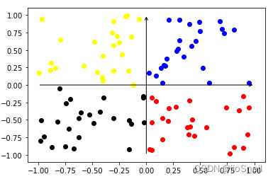
这里我们定义100个样本,每个样本有两个特征(x, y),Label有(0,1,2,4),即所属的象限:
```python
samples = torch.rand(100, 2)
samples[25:50, 0] -= 1
samples[50:75, :] -= 1
samples[75:100, 1] -= 1
labels = torch.LongTensor([0] * 25 + [1] * 25 + [2] * 25 + [3] * 25)
```
绘制我们的样本,如下:
```python
plot_samples(samples, labels)
```
之后我们定义一个encoder来模拟卷积网络、BERT等负责提取特征的backbone:
```python
encoder = nn.Sequential(
    nn.Linear(2, 10, bias=False),
    nn.Linear(10, 2, bias=False),
    nn.Tanh()
)
```
经过encoder后,我们会提取样本的特征,绘制到图中如下:
```python
plot_samples(encoder(samples).clone().detach(), labels)
```
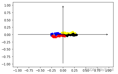
从图上我们可以看到我们的encoder提取的特征都挤在一起了,这对于后续网络的分类很不利,所以对比学习就派上用场了,让相似的样本离得近一点,不相似的样本距离远一点,最终可以做到均匀分布。
这里举得例子不够好,因为相似样本距离已经很近了。
我们首先准备一下使用对比学习训练encoder的代码:
```python
def train_and_plot(step=10000, temperature=0.05):
    """
    step: 训练次数
    temperature:温度系数
    """
    encoder_ = copy.deepcopy(encoder) # 这里复制一个encoder,别污染原来的encoder,因为后面要做对比实验
    loss_fnt = nn.CrossEntropyLoss()
    optimizer = torch.optim.SGD(encoder_.parameters(), lr=3e-4)

    # 训练step次,简单期间,这里batch_size=1
    for _ in tqdm(range(step)):
        anchor_label = random.randint(0, 3)   # 从4个label里随机挑出一种作为anchor
        anchor_sample = samples[labels == anchor_label][random.sample(range(25), 1)]  # 从anchor样本中随机挑出一个样本
        positive_sample = samples[labels == anchor_label][random.sample(range(25), 1)] # 从anchor样本中再挑出一个做成正样本
        negative_samples = samples[labels != anchor_label][random.sample(range(75), 3)] # 从其他样本中挑出3个作为负样本

        # 使用encoder提取各个样本的特征
        anchor_feature = encoder_(anchor_sample)
        positive_feature = encoder_(positive_sample)
        negative_feature = encoder_(negative_samples)

        # 计算anchor与正样本和负样本的相似度
        positive_sim = F.cosine_similarity(anchor_feature, positive_feature)
        negative_sim = F.cosine_similarity(anchor_feature, negative_feature)

        # 将正样本和负样本concat起来,再除以温度参数
        sims = torch.concat([positive_sim, negative_sim]) / temperature
        # 构建CrossEntropyLoss的Label,因为我把正样本放在了第0个位置,所以Label为0
        sims_label = torch.LongTensor([0])

        # 计算CrossEntropyLoss
        loss = loss_fnt(sims.unsqueeze(0), sims_label.view(-1))
        loss.backward()
        # 更新参数
        optimizer.step()
        optimizer.zero_grad()

    # 绘制训练后的结果。
    plot_samples(encoder_(samples).clone().detach(), labels)
```
接下来使用0.05的温度参数训练一下encoder,然后重新绘制samples的特征向量:
```python
train_and_plot(10000, temperature=0.05)
```
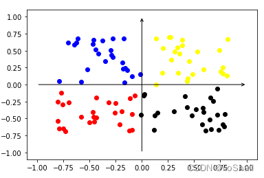
可以看到,经过对比学习后,特征分布更加均匀了。
3. 对比学习不同温度系数比较
上一节我们准备了一个对比学习的训练函数,所以只需要使用不同的参数就能进行比较:
```python
train_and_plot(10000, temperature=0.99)
train_and_plot(10000, temperature=0.5)
train_and_plot(10000, temperature=0.05)
train_and_plot(10000, temperature=0.01)
train_and_plot(10000, temperature=0.001)
```
最终我们得到如下图:
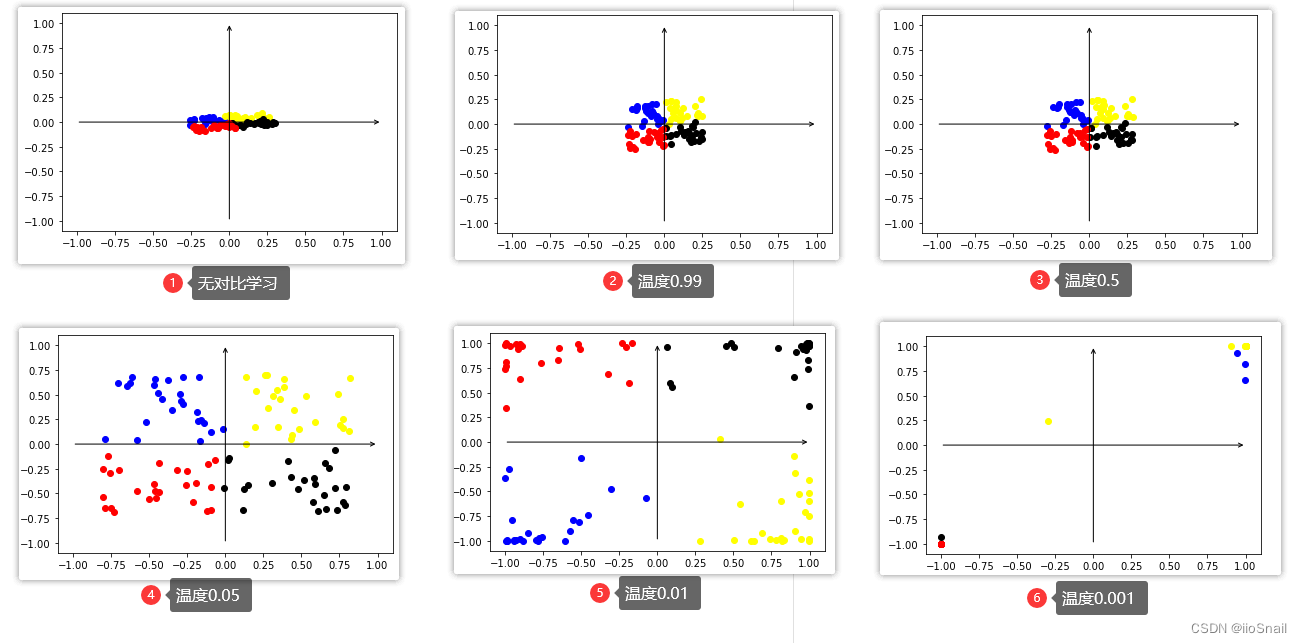
最后的0.001温度系数点看起来很少并不是因为点消失或出界了,而是因为网络使用了Tanh激活函数,将特征限制在了(-1, 1)之间,所以样本点都集中在了 $(-1, 1)$ 和 $(-1, -1)$ 这两个位置。
结论
从上图中可以看出如下结论:
- 温度参数越小,对比学习效果越强,即对比学习让相似样本距离就会越近,不相似样本距离越远
- 若想要让样本特征分布均匀,温度参数需要适中,太大和太小都不好。
4. 对比学习结论分析
之所以会出现上述的结果,其实很容易分析,我们只需要看一下不同参数的求Loss过程中的变化即可。
假设我们的锚点样本和正负样本的相似度如下:
$[\text{sim}(x, x'_1), \text{sim}(x, y_2), \text{sim}(x, y_3), \text{sim}(x, y_4)]$ = [0.5, 0.25, -0.45, -0.1]
我们来看一下随着温度参数的变化,相似度、SoftMax的概率分布和CrossEntropyLoss都是如何变化的:
| 温度 | sim | Softmax概率分布 | CrossEntropyLoss |
|---|---|---|---|
| 1 | [0.5, 0.25, -0.45, -0.1] | [0.3684, 0.2869, 0.1425, 0.2022] | 0.9986 |
| 0.5 | [ 1.0, 0.5, -0.9, -0.2] | [0.4861, 0.2948, 0.0727, 0.1464] | 0.7214 |
| 0.05 | [10, 5, -9, -2] | [0.9933, 6.6e-03, 5.5e-09, 6.1-06] | 0.0067 |
| 0.01 | [ 50, 25, -45, -10] | [1.00, 1.3e-11, 5.5-42, 8.7-27] | 0 |
你可以使用下面这段代码进行上述表格的实验:
```python
t = 1   # 温度参数
sims = torch.tensor([0.5, 0.25, -0.45, -0.1]) / t
print(sims)
prob = F.softmax(sims, dim=-1)
print(prob)
loss = F.cross_entropy(sims.unsqueeze(0), torch.LongTensor([0]))
print(loss)
```
从上面的表格可以得到如下结论:
- 温度系数越低,概率分布就越陡。也就是在对比学习中经常看到的图:
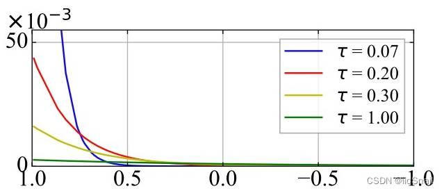
这个图可能看起来还不够清晰,如果用正态分布表示,则为:
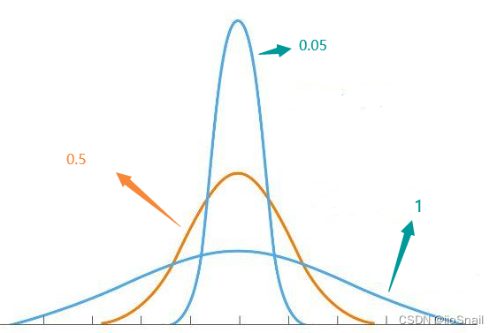
(此图并不严谨,是随便画的,主要用于感受温度变化对概率分布的调整) - 当锚点与正样本的相似度最高时,温度系数越低,loss越低。
上述表格是假设了锚点与正样本的相似度最高,若锚点与某个负样本相似度低呢?
假设我们的锚点样本和正负样本的相似度如下:
$[\text{sim}(x, x'_1), \text{sim}(x, y_2), \text{sim}(x, y_3), \text{sim}(x, y_4)]$ = [0.25, 0.5, -0.45, -0.1]
那么,随着温度参数的变化,相似度、SoftMax的概率分布和CrossEntropyLoss都是如何变化的:
| 温度 | sim | Softmax概率分布 | CrossEntropyLoss |
|---|---|---|---|
| 1 | [0.25, 0.5, -0.45, -0.1] | [0.2869, 0.3684, 0.1425, 0.2022] | 1.2486 |
| 0.5 | [ 0.5, 1.0, -0.9, -0.2] | [0.2948, 0.4861, 0.0727, 0.1464] | 1.2214 |
| 0.05 | [5, 10, -9, -2] | [ 6.6e-03, 0.9933, 5.5e-09, 6.1-06] | 5.0067 |
| 0.01 | [ 25, 50, -45, -10] | [1.3e-11, 1.00, 5.5-42, 8.7-27] | 25 |
通过这两个表格,我们可以得到温度系数与Loss的关系:
- 当锚点与正样本的相似度最高时,温度系数越低,loss越低。
- 当锚点与某个负样本的相似度最高时,温度系数越低,loss越高。
- 由1可知,当温度系数较高时,模型的调节相对温和,不论模型是否正确预测正样本,都会调节模型
- 由2可知,当温度系数较低时,模型的调节比较锐利,模型偏向尽快学会预测正样本,学会后就几乎不再调节模型。
5. 温度系数结论
上述结论都是根据自己的理解与实验得出的,若有不严谨或错误的地方请各位在评论区指出。
温度系数的不同取值有以下结论:
- 温度参数越小,对比学习效果越强,即对比学习让相似样本距离就会越近,不相似样本距离越远
- 若想要让样本特征分布均匀,温度参数需要适中,太大和太小都不好。
- 当锚点与正样本的相似度最高时,温度系数越低,loss越低。
- 当锚点与某个负样本的相似度最高时,温度系数越低,loss越高。
- 由1可知,当温度系数较高时,模型的调节相对温和,不论模型是否正确预测正样本,都会调节模型
- 由4可知,当温度系数较低时,模型的调节比较锐利,模型偏向尽快让学会预测正样本,学会后就几乎不再调节模型。
1,2结论请参考第3节。3,4,5,6结论请参考第4节。
常用的温度系数是 0.05
