Stochastic Weight Averaging (SWA) and its Implementation in PyTorch Lightning
Table of Content
Introduction to SWA
SWA, short for "Stochastic Weight Averaging," is a popular technique in deep learning used to enhance model generalization.
The core idea is this: Instead of using the final model weights directly, SWA averages the weights from several earlier training stages.
SWA can be applied in various deep learning fields and is compatible with different optimizers, making it versatile enough to work alongside other training techniques.
SWA Formula
Let's denote our model parameters as :$\theta=\{w_0, w_1, w_2, \cdots, w_n\}$, where $n$ represents the total number of parameters.
During training, we save a copy of model parameters at the end of each epoch. Let's $\theta_t$ represents the model parameters at epoch $t$.
The final parameters are calculated as:
$$ \begin{aligned} \bar{\theta} = \frac{1}{T} \sum^T_{t=1}\theta_t \end{aligned} $$
where $T$ indicates the total number of saved model parameter
In essence, the formula means that the final model parameters are an average of the weights from all checkpoints.
Considerations:
- Typically, model parameters are only saved at the end of each epoch.
- You don't need to save model parameters every epoch. Usually, checkpoints start only once the model begins to converge well.
Common SWA Hyperparameters
When using SWA, there are usually a few key hyperparamters to set:
- SWA Start:Specifies from which epoch to start saving model checkpoints. Saving checkpoints too early, before the model has started converging, could reduce performance.
- SWA Learning Rate:The learing rate used during SWA. For instance, if SWA starts at epoch 20, the SWA Learning Rate will be applied from epoch 20 onward, replacing the previous learning rate.
Source Code Analysis of SWA in PyTorch Lightning
This section explores the implementation of Stochastic Weight Averaging (SWA) in PyTorch Lightning to provide a clearer understanding of SWA.
Before examining the code, let's clarify a few key concepts used in PyTorch Lightning’s SWA implementation:
- Average Model(
self._average_model):PyTorch Lightning stores the averaged model in this variable. pl_module:This variable represents the current model.
```python
class StochasticWeightAveraging(Callback):
    def __init__(
        self,
        swa_lrs: Union[float, List[float]],  # Learning rate for SWA
        # swa_epoch_start: Defines the starting point for SWA, at 80% by default.
        #                 For example, if there are 100 epochs in total, SWA starts at epoch 81.
        #                 You can also specify a particular epoch number to start SWA.
        swa_epoch_start: Union[int, float] = 0.8,
        annealing_epochs: int = 10,  # Number of epochs for annealing, used by SWALR strategy
        annealing_strategy: str = "cos",  # Annealing strategy for SWALR, e.g., cosine
        avg_fn: Optional[_AVG_FN] = None,  # Averaging function for model parameters; defaults to built-in function
        device: Optional[Union[torch.device, str]] = torch.device("cpu"),  # Device for the averaged model
    ):
    ...

    def on_train_epoch_start(self, ...):  # Executes at the start of each epoch
        if (not self._initialized) and (self.swa_start <= trainer.current_epoch <= self.swa_end):
            # Initialize SWA, only runs once throughout SWA
            self._initialized = True
            ...

            # Use the original optimizer
            optimizer = trainer.optimizers[0]

            ...

            # Apply SWALR learning rate scheduler (explained below)
            self._swa_scheduler = cast(
                LRScheduler,
                SWALR(
                    optimizer,
                    swa_lr=self._swa_lrs,  # type: ignore[arg-type]
                    anneal_epochs=self._annealing_epochs,
                    anneal_strategy=self._annealing_strategy,
                    last_epoch=trainer.max_epochs if self._annealing_strategy == "cos" else -1,
                ),
            )

        # End of initialization code.

        # SWA processing logic at the start of each epoch
        if (self.swa_start <= trainer.current_epoch <= self.swa_end):
            # During SWA, update model parameters to the “averaged model” at the start of each epoch
            self.update_parameters(self._average_model, pl_module, self.n_averaged, self._avg_fn)

        if trainer.current_epoch == self.swa_end + 1:
            # At the end, transfer averaged model parameters back to the model
            self.transfer_weights(self._average_model, pl_module)

    @staticmethod
    def update_parameters(
        average_model: "pl.LightningModule", model: "pl.LightningModule", n_averaged: Tensor, avg_fn: _AVG_FN
    ) -> None:
        for p_swa, p_model in zip(average_model.parameters(), model.parameters()):
            device = p_swa.device
            p_swa_ = p_swa.detach()
            p_model_ = p_model.detach().to(device)
            src = p_model_ if n_averaged == 0 else avg_fn(p_swa_, p_model_, n_averaged.to(device))
            p_swa_.copy_(src)
        n_averaged += 1

    @staticmethod
    def avg_fn(averaged_model_parameter: Tensor, model_parameter: Tensor, num_averaged: Tensor) -> Tensor:
        return averaged_model_parameter + (model_parameter - averaged_model_parameter) / (num_averaged + 1)
```
From the source code, we can gather the following insights about SWA in PyTorch Lightning:
- Using SWA requires specifying two critical parameters: the SWA learning rate and the epoch from which SWA should start.
- Once SWA begins, a new learning rate (
swa_lrs) and a new learning rate schedule (SWALR) are used. However, the model’s original learning rate is referenced during the "annealing" phase. - At the beginning of each epoch, the model parameters learned from the previous epoch are updated into the "average model."
- During SWA, the optimizer remains the same as used in prior training. For instance, if Adam was used during training, Adam will also be used during SWA.
SWALR
As mentioned above, in the PyTorch Lightning implementation, SWALR is used during the Stochastic Weight Averaging (SWA) process.
SWALR adopts an "annealing" strategy, which gradually transitions the learning rate from the original learning rate to the SWA learning rate. For example, if the initial learning rate is 0.1, and the designated SWA learning rate is 0.01, with SWA starting from the 20th epoch, the learning rate doesn’t instantly change from 0.1 to 0.01. Instead, it gradually shifts down to 0.01 over a period defined by the annealing_epochs parameter, following a reduction pattern specified by the annealing_strategy parameter.
Instead of delving into complex code or mathematics, we’ll visually explore how the learning rate changes under the SWALR (Stochastic Weight Averaging with Learning Rate Rescheduling) strategy through a series of experiments:
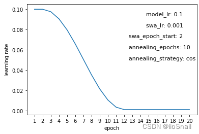
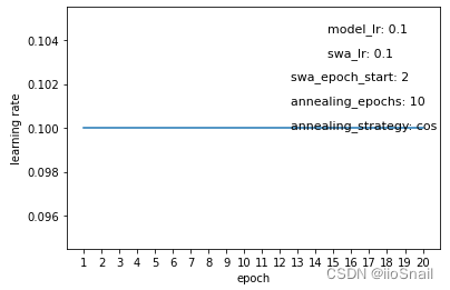
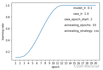
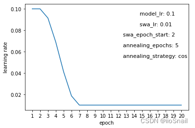
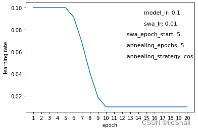
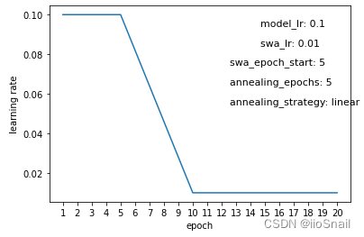
The experiment above illustrates the changes in learning rate throughout the training process, where the x-axis represents the epochs, and the y-axis shows the learning rate used at each epoch. Key parameters represented in these graphs include:
model_lr:The initial learning rate of the model.swa_lr:The user-defined learning rate for SWA.swa_epoch_start:The epoch at which SWA begins.annealing_epoch:Number of epochs used for annealing.annealing_strategy:The strategy for annealing. Currently, only “cos” (cosine) and “linear” strategies are supported.

As shown in Figure 1, the initial learning rate set in the optimizer for the model is 0.1, while the SWA (Stochastic Weight Averaging) learning rate is 0.001. Starting from the 2nd epoch, SWA is applied, and the learning rate transitions from 0.1 to 0.001 over 10 epochs (annealing_epochs) using a cosine strategy.
From the figure, we can draw a few conclusions:
- The SWALR strategy gradually adjusts the learning rate from the original rate to the SWA learning rate, with the number of transition epochs defined by
annealing_epochs. - If the SWA learning rate is set to the same value as the initial learning rate, SWALR effectively has no impact (Figure 2).
- If the SWA learning rate is higher than the original rate, the learning rate will increase gradually (Figure 3). However, this is rarely done; typically, the SWA learning rate is lower than the model's original rate since the model stabilizes over time and higher rates are unsuitable.
- If the
annealing_epochscount is low, the "annealing" process is faster, meaning the transition frommodel_lrtoswa_lris quicker (Figure 4); with more epochs, the transition is slower. - With the cosine annealing strategy, the rate change is slow at first, then quick, and slows again at the end (Figure 5). With a linear strategy, the rate change is consistent throughout (Figure 6).
The experiment environment and code are as follows:
```python
lightning==2.0.1
pytorch==1.13.0
```
```python
import torch
import torch.nn as nn

import lightning.pytorch as pl
from lightning.pytorch.callbacks import StochasticWeightAveraging

from matplotlib import pyplot as plt

import numpy as np

def plot_swa_lr_curve(model_lr,  # Model's learning rate
                      swa_lr,  # SWA's learning rate
                      swa_epoch_start=2,  # Starting epoch for SWA
                      annealing_epochs=10,  # Number of epochs for simulated annealing
                      annealing_strategy='cos'  # Annealing strategy
                      ):
    lrs = []

    # Define a simple model for testing
    class SimpleModel(pl.LightningModule):

        def __init__(self):
            super(SimpleModel, self).__init__()
            self.linear = nn.Linear(1, 1)

        def training_step(self, batch, batch_idx, *args, **kwargs):
            return nn.functional.mse_loss(self.linear(torch.rand(4, 1)), torch.rand(4, 1))

        def configure_optimizers(self):
            # Use model_lr as the learning rate for the test model
            return torch.optim.SGD(self.parameters(), lr=model_lr)

    # Override StochasticWeightAveraging to record learning rate changes
    class MyStochasticWeightAveraging(StochasticWeightAveraging):

        def on_train_epoch_start(self, *args, **kwargs):
            super().on_train_epoch_start(*args, **kwargs)
            if hasattr(self._swa_scheduler, "_last_lr"):
                # Record the learning rate changes
                lrs.append(self._swa_scheduler._last_lr[0])
            else:
                lrs.append(model_lr)

    # Define a trainer to train the model
    trainer = pl.Trainer(
        callbacks=[MyStochasticWeightAveraging(swa_lrs=swa_lr, swa_epoch_start=swa_epoch_start,
                                               annealing_epochs=annealing_epochs,
                                               annealing_strategy=annealing_strategy)],
        max_epochs=20,
        num_sanity_val_steps=0,
        enable_progress_bar=False,  # Use custom progress bar
        accelerator='cpu',
    )

    # Train the model
    trainer.fit(SimpleModel(), train_dataloaders=range(10))

    plt.plot(np.arange(1, len(lrs)+1).astype(dtype=np.str), lrs)
    plt.xlabel("epoch")
    plt.ylabel("learning rate")
    plt.text(0.7, 0.9, "model_lr: %s" % model_lr, fontsize=11, transform=plt.gca().transAxes)
    plt.text(0.7, 0.8, "swa_lr: %s" % swa_lr, fontsize=11, transform=plt.gca().transAxes)
    plt.text(0.6, 0.7, "swa_epoch_start: %s" % swa_epoch_start, fontsize=11, transform=plt.gca().transAxes)
    plt.text(0.6, 0.6, "annealing_epochs: %s" % annealing_epochs, fontsize=11, transform=plt.gca().transAxes)
    plt.text(0.6, 0.5, "annealing_strategy: %s" % annealing_strategy, fontsize=11, transform=plt.gca().transAxes)
    plt.show()

    print("lrs:", lrs)  # Output the learning rate changes
    return lrs

plot_swa_lr_curve(0.1, 0.001)
```
References
Averaging Weights Leads to Wider Optima and Better Generalization(原论文): https://arxiv.org/abs/1803.05407
PyTorch 1.6 now includes Stochastic Weight Averaging: https://pytorch.org/blog/pytorch-1.6-now-includes-stochastic-weight-averaging/


