中文 | English

Overview

This article is based on Li Hongyi's lecture on Self-Attention, expanding upon his explanations and incorporating additional understanding and PyTorch code examples. The goal is to help both myself and readers develop a clearer understanding of Self-Attention.

Link to Li Hongyi's Self-Attention Lecture: https://www.youtube.com/watch?v=hYdO9CscNes

Slides can be found below the video.

After reading this article, you should gain the following insights:

• What Self-Attention is and why we use it
• How Self-Attention works
• How Self-Attention is designed
• Detailed explanation of the Self-Attention formula
• MultiHead Attention
• Masked Attention

1、Self-Attention

1.1. Why Use Self-Attention

Let’s consider a part-of-speech tagging (POS tagging) task as an example. Suppose the input is the sentence I saw a saw, and our goal is to identify the part of speech for each word, resulting in N, V, DET, N (Noun, Verb, Determiner, Noun).

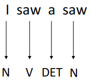
In this sentence, the first saw is a verb, while the second saw refers to a noun (a saw). To make this distinction, the model needs to consider the context surrounding each word and determine how much attention each context element should receive. For example, when processing the first saw, the model should focus more on I, while for the second saw, it should give more attention to a.

This is where the Attention mechanism comes in: if a task involves an input sequence (a series of vectors) with interdependent relationships, then the Attention mechanism helps capture these relationships.

1.2. A Closer Look at Self-Attention

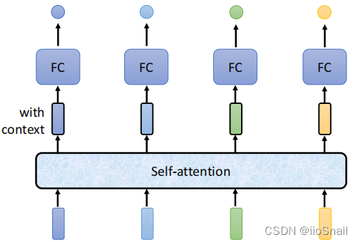
This illustration shows how Self-Attention works. Self-Attention takes in a sequence (a series of vectors, which could be inputs or outputs from a previous hidden layer) and outputs a sequence of the same length, where each vector incorporates context from the entire sequence.

For instance, if the input sequence is I, saw, a, saw, represented by vectors as follows:

$$\begin{array}{r}\text{I}=\left[\begin{array}{c}1\\ 0\\ 0\end{array}\right],\text{saw}=\left[\begin{array}{c}0\\ 1\\ 0\end{array}\right],\text{a}=\left[\begin{array}{c}0\\ 0\\ 1\end{array}\right],\text{saw}=\left[\begin{array}{c}0\\ 1\\ 0\end{array}\right]\end{array}$$

After passing through the Self-Attention layer, the sequence might be transformed to something like this:

$$\begin{array}{r}{\text{I}}^{\prime }=\left[\begin{array}{c}0.7\\ 0.28\\ 0.02\end{array}\right],{\text{saw}}^{\prime }=\left[\begin{array}{c}0.34\\ 0.65\\ 0.01\end{array}\right],{\text{a}}^{\prime }=\left[\begin{array}{c}0.2\\ 0.2\\ 0.6\end{array}\right],{\text{saw}}^{\prime }=\left[\begin{array}{c}0.01\\ 0.5\\ 0.49\end{array}\right]\end{array}$$

In this transformed sequence, the first instance of saw now reflects $0.34$ of I, while the second saw incorporates $0.49$ of a to capture contextual meaning.

1.3. How Self-Attention Incorporates Context?

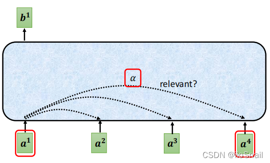
As shown, each input vector is compared with all others in the sequence to calculate a relevance score, which is used to generate a new, contextually enriched vector.

For example, to calculate the new representation for $a^1$, we determine its relevance scores ${\alpha }_{1,1},{\alpha }_{1,2},{\alpha }_{1,3},{\alpha }_{1,4}$ with respect to $a^1,a^2,a^3,$ and $a^4$ (including itself). The higher the $\alpha$ score, the more relevant the two vectors are to each other.

Once we have these ${\alpha }_{1,\ast }$ values, we can create a new vector $b^1$ that captures context, based on scores like ${\alpha }_{1,1}=5,{\alpha }_{1,2}=2,{\alpha }_{1,3}=1,{\alpha }_{1,4}=2$, resulting in:

$$\begin{array}{r}{b}_1=\sum _i{\alpha }_{1,i}\cdot a^i=5\cdot a^1+2\cdot a^2+1\cdot a^3+2\cdot a^4\end{array}$$

Similarly, to compute $b_2$, we would first find the weights ${\alpha }_{2,1},{\alpha }_{2,2},{\alpha }_{2,3},{\alpha }_{2,4}$ and then perform a weighted sum.

There are two common issues when computing this way:

1. The sum of the $\alpha$ values might not be 1, which could scale the input vectors up or down unpredictably.
2. Directly multiplying by the input vector $a^i$ can limit the model's expressive power.

To address these issues:

• For issue 1, we often apply a Softmax function to the $\alpha$ values (though other methods are possible).
• For issue 2, we typically multiply $a^i$ by a learnable matrix to create $v^i$, which is then weighted by the $\alpha$ values.

1.4. How to Calculate the Relevance Score $\alpha$

First, let’s review vector multiplication. When two vectors are multiplied (taking their inner product), the formula is: $a\cdot b=|a||b|\cos \theta$. From this formula, we can conclude:

• The smaller the angle between two vectors (the more aligned they are), the larger the inner product, and the higher the relevance. Conversely, the larger the angle, the less relevant they are. If the angle is 90°, the vectors are perpendicular, giving an inner product of 0, indicating no relevance.

From this, it seems straightforward to measure the relevance of $a^1$ and $a^2$ by directly calculating their inner product, i.e., ${\alpha }_{1,2}=a_1\cdot a_2$. However, this simple approach has issues. For instance, in the sentence "I saw a saw," the word "saw" would be highly relevant to itself (two identical vectors have an angle of 0), which doesn’t accurately capture context.

To address this, Self-Attention introduces two additional matrices, $W^q$ and $W^k$, which serve specific functions:

• $W^q$ applies a linear transformation to the “main word” or “query” to produce $q$, referred to as the query vector.
• $W^k$ applies a linear transformation to the “context word” or “key” to produce $k$, referred to as the key vector.

With $W^q$ and $W^k$, we can now compute the relevance score ${\alpha }_{1,2}$ between $a^1$ and $a^2$ as follows:

$$\begin{array}{r}{\alpha }_{1,2}=q^1\cdot k^2=(W^q\cdot a^1)\cdot (W^k\cdot a^2)\end{array}$$

This process is summarized visually in the diagram below:

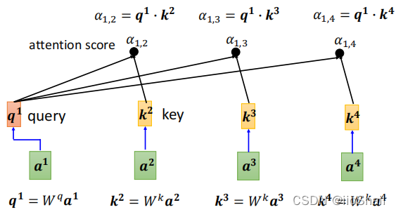
To calculate the relevance between $a^1$ (main term) and $a^1,a^2,a^3,a^4$ (context terms), the following steps are needed:

1. Use $W^q$ to compute $q^1$
2. Use $W^k$ to compute $k^1,k^2,k^3,k^4$
3. Calculate ${\alpha }_{1,1},{\alpha }_{1,2},{\alpha }_{1,3},{\alpha }_{1,4}$ using $q$ and $k$ values

The diagram doesn’t explicitly show $k^1$, but in actual calculations, we include $k_1$, meaning we also calculate the relevance score between $a^1$ and itself.

1.5. Normalizing $\alpha$

As we mentioned earlier, the sum of $\alpha$ values is not equal to 1. Therefore, after calculating ${\alpha }_{1,\ast }$, we still need to apply a Softmax function to normalize ${\alpha }_{1,\ast }$, as shown in the diagram below:

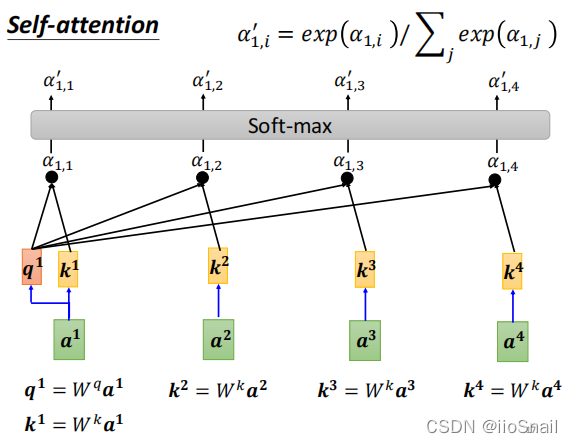
In the end, the normalized ${\alpha }_{1,}^{\prime }$ will be used as the relevance score of $a^1$ with respect to other vectors. Similarly, the relevance scores for vectors $a^2,a^3,...$ in relation to other vectors are calculated in the same way.

It's not mandatory to use Softmax—feel free to try any other method if you think it might work better. Normalization isn’t strictly required either, although it’s commonly applied in practice.

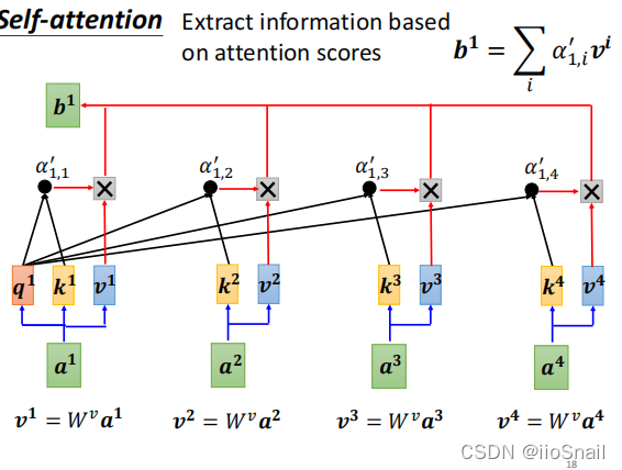
1.6. Combining All the Components

Once we have computed the attention scores ${\alpha }^{\prime }$, we can proceed to a weighted sum to calculate the context-aware vector $b$. Recall that if we directly use $\alpha$ with ${\alpha }^{\prime }$ for the weighted sum, the model’s generalization ability might be limited. Therefore, we apply a linear transformation to $\alpha$ to get a new vector $v$. This requires training an additional matrix $W^v$ to perform the linear transformation on $\alpha$, as shown below:

$$\begin{array}{r}{v}^1=W^v\cdot a^1{v}^2=W^v\cdot a^2{v}^3=W^v\cdot a^3{v}^4=W^v\cdot a^4\end{array}$$

After obtaining $v$, we can use it along with ${\alpha }^{\prime }$ in the weighted sum to compute $b$:

$$\begin{array}{r}{b}^1=\sum _i{\alpha }_{1,i}^{\prime }\cdot v^i={\alpha }_{1,1}^{\prime }\cdot v^1+{\alpha }_{1,2}^{\prime }\cdot v^2+{\alpha }_{1,3}^{\prime }\cdot v^3+{\alpha }_{1,4}^{\prime }\cdot v^4\end{array}$$

The process of computing $b^1$ is summarized in the diagram below:

To formally describe the process:

Given an input sequence $I=(a^1,a^2,\cdots ,a^n)$，where each $a^i$ is a vector, the Self-Attention mechanism transforms it into a new sequence $O=(b^1,b^2,\cdots ,b^n)$. Each vector $b^i$ is derived from $a^i$ combined with its contextual information.. The process of calculating $b^i$ is as follows:

1. Compute the query vector $q^i$ using the formula $q^i=W^q\cdot a^i$
2. Calculate $k^1,k^2,\cdots ,k^n$, where $k^j=W^k\cdot a^j$
3. Compute attention scores ${\alpha }_{i,1},{\alpha }_{i,2},\cdots ,{\alpha }_{i,n}$ using the formula ${\alpha }_{i,j}=q^i\cdot k^j$
4. Normalize ${\alpha }_{i,1},{\alpha }_{i,2},\cdots ,{\alpha }_{i,n}$ to obtain ${\alpha }_{i,1}^{\prime },{\alpha }_{i,2}^{\prime },\cdots ,{\alpha }_{i,n}^{\prime }$ with the formula ${\alpha }_{i,j}^{\prime }=\text{Softmax}({\alpha }_{i,j};{\alpha }_{i,\ast })=\exp ({\alpha }_{i,j})/\sum _t\exp ({\alpha }_{i,t})$
5. Obtain vectors $v^1,v^2,\cdots ,v^n$ using the formula $v^j=W^v\cdot a^j$
6. Calculate $b^i$ with the formula $b^i=\sum _j{\alpha }_{i,j}^{\prime }\cdot v^j$

Here, $W^q,W^k,W^v$ are trainable parameters.

---

While the Self-Attention mechanism is now clearer, there's an additional step. The above calculations, if implemented directly in code, would require numerous for-loops, which would be computationally inefficient. To improve efficiency, vectorization is necessary, merging components into vectors and matrices wherever possible.

1.7. Vectorization

To begin, let's consider vectorizing a vector $a$. Assume that each vector $a^i$ is a column vector of dimension $d$. It is possible to arrange all input vectors into a single matrix $I$ as follows:

$$\begin{array}{r}{I}_{d\times n}=(a^1,a^2,\cdots ,a^n)\end{array}$$

Next, we define the matrices $W^q,W^k$ and $W^v$ . The matrices $W^q$ and $W^k$ must have the same dimensions, specifically $d_k\times d$, while $W^v$ has dimensions $d_v\times d$. Here, $d_k$ and $d_v$ are hyperparameters that can be tuned, typically matching the dimension $d$ of the word embeddings. While $d_k$ only affects the calculation process, $d_v$ directly impacts the output because it determines the dimension of the Attention output vector $b$.

Once we’ve defined the dimensions of $W^q$, we can proceed to matrix the vector $q$.

The matrix form of $q$ is given by:

$$\begin{array}{r}{Q}_{d_k\times n}=(q^1,q^2,\cdots ,q^n)=W_{d_k\times d}^q\cdot I_{d\times n}\end{array}$$

Similarly, the matrix form of $k$ is:

$$\begin{array}{r}{K}_{d_k\times n}=(k^1,k^2,\cdots ,k^n)=W^k\cdot I\end{array}$$

Likewise, the matrix form of $v$ is:

$$\begin{array}{r}{V}_{d_v\times n}=(v^1,v^2,\cdots ,v^n)=W^v\cdot I\end{array}$$

With matrices $Q$ and $K$ in hand, we can now compute the matrix form of the relevance score $\alpha$.

The matrix form of the relevance score $\alpha$ is as follows:

$$\begin{array}{r}{A}_{n\times n}=\left[\begin{array}{cccc}{\alpha }_{1,1}& {\alpha }_{2,1}& \cdots & {\alpha }_{n,1}\\ {\alpha }_{1,2}& {\alpha }_{2,2}& \cdots & {\alpha }_{n,2}\\ ⋮& ⋮& & ⋮\\ {\alpha }_{1,n}& {\alpha }_{2,n}& \cdots & {\alpha }_{n,n}\end{array}\right]=K^T\cdot Q=\left[\begin{array}{c}{k^1}^T\\ {k^2}^T\\ ⋮\\ {k^n}^T\end{array}\right]\cdot (q^1,q^2,\cdots ,q^n)\end{array}$$

Note: I defined $k^i$ as a column vector, so we will transpose it.

Then, we can calculate an adjusted matrix ${\alpha }^{\prime }$：

$$\begin{array}{r}{A}_{n\times n}^{\prime }=\mathbf{\text{softmax}}(A)=\left[\begin{array}{cccc}{\alpha }_{1,1}^{\prime }& {\alpha }_{2,1}^{\prime }& \cdots & {\alpha }_{n,1}^{\prime }\\ {\alpha }_{1,2}^{\prime }& {\alpha }_{2,2}^{\prime }& \cdots & {\alpha }_{n,2}^{\prime }\\ ⋮& ⋮& & ⋮\\ {\alpha }_{1,n}^{\prime }& {\alpha }_{2,n}^{\prime }& \cdots & {\alpha }_{n,n}^{\prime }\end{array}\right]\end{array}$$

Once we have $A^{\prime }$ and $V$, we can vectorize the output vector $b$.

The matrix form for vectorizing $b$ is

$$\begin{array}{r}{O}_{d_v\times n}=(b^1,b^2,\cdots ,b^n)=V_{d_v\times n}\cdot A_{n\times n}^{\prime }=(v^1,v^2,\cdots ,v^n)\cdot \left[\begin{array}{cccc}{\alpha }_{1,1}^{\prime }& {\alpha }_{2,1}^{\prime }& \cdots & {\alpha }_{n,1}^{\prime }\\ {\alpha }_{1,2}^{\prime }& {\alpha }_{2,2}^{\prime }& \cdots & {\alpha }_{n,2}^{\prime }\\ ⋮& ⋮& & ⋮\\ {\alpha }_{1,n}^{\prime }& {\alpha }_{2,n}^{\prime }& \cdots & {\alpha }_{n,n}^{\prime }\end{array}\right]\end{array}$$

Bringing it all together, we can derive the final combined equation:

$$\begin{array}{r}O=\mathbf{\text{Attention}}(Q,K,V)=V\cdot \mathbf{\text{softmax}}(K^{T}Q)\end{array}$$

If you’ve seen other resources on this topic, you may notice that the actual final formula is as follows:

$$\begin{array}{r}\text{ Attention }(Q,K,V)=\mathrm{softmax}\left(\frac{Q{K}^T}{\sqrt{d_k}}\right)V\end{array}$$

Our formula differs only by a transpose and the factor $\sqrt{d_k}$. The transpose merely reflects a different notation.

In the original formula, the matrices $Q,K,V$ , and the output $O$ correspond to $Q^T,K^T,V^T$, and $O^T$ in our formula, respectively.

1.8. What is $d_k$ and Why Divide by $\sqrt{d_k}$

Firstly, $d_k$ is the row dimension of the Q and K matrices, specifically the $d_k$ in $Q_{d_k\times d}$ above. When matrices are multiplied, the standard deviation of the result is amplified by approximately $\sqrt{d_k}$. To normalize the standard deviation back to its original scale, we divide by $\sqrt{d_k}$.

For example, assume $Q_{n\times d_k}$ and $K_{n\times d_k}$ have a mean of 0 and a standard deviation of 1. Then, the matrix $Q{K}^T$ will have a mean of 0 but a standard deviation of $\sqrt{d_k}$, indicating that the multiplication has amplified the standard deviation by a factor of $\sqrt{d_k}$.

The mean of a matrix is simply the sum of all its elements divided by the total number of elements, and variance follows similarly.

This effect can be confirmed through the following code (since my math is weak, I’m validating with an experiment—sigh):

```python
Q = np.random.normal(size=(123, 456)) # Generate Q and K with mean 0, std 1
K = np.random.normal(size=(123, 456))
print("Q.std=%s, K.std=%s, \nQ·K^T.std=%s, Q·K^T/√d.std=%s" 
      % (Q.std(), K.std(), 
         Q.dot(K.T).std(), Q.dot(K.T).std() / np.sqrt(456)))
```

```
Q.std=0.9977961671085275, K.std=1.0000574599289282,
Q·K^T.std=21.240017020263437, Q·K^T/√d.std=0.9946549289466212
```

From the output, we can see that the standard deviations of Q and K are both around 1, but after multiplying the matrices, the standard deviation rises to 21.24. Dividing by $\sqrt{d_k}$ brings the standard deviation back to approximately 1.

Here's another example where Q and K have random standard deviations, which is closer to a real-world scenario:

```python
Q = np.random.normal(loc=1.56, scale=0.36, size=(123, 456)) # Generate Q and K with random mean and std
K = np.random.normal(loc=-0.34, scale=1.2, size=(123, 456))
print("Q.std=%s, K.std=%s, \nQ·K^T.std=%s, Q·K^T/√d.std=%s" 
      % (Q.std(), K.std(), 
         Q.dot(K.T).std(), Q.dot(K.T).std() / np.sqrt(456)))
```

```
Q.std=0.357460640868945, K.std=1.204536717914841, 
Q·K^T.std=37.78368871510589, Q·K^T/√d.std=1.769383337989377
```

In this case, the initial standard deviations of Q and K are $0.35$ and $1.20$, respectively. After matrix multiplication, the standard deviation increases to $37.78$, but after scaling, it returns to $1.76$.

1.9. Code Practice: Defining a Self-Attention Model in PyTorch

Let's define a Self-Attention model in PyTorch using the original formula from the attention mechanism paper:

$$\begin{array}{r}\text{ Attention }(Q,K,V)=\mathrm{softmax}\left(\frac{Q{K}^T}{\sqrt{d_k}}\right)V\end{array}$$

To make the code logic clearer, I've labeled the dimensions of each component:

$$\begin{array}{rl}{O}_{n\times d_v}=\text{ Attention }(Q_{n\times d_k},K_{n\times d_k},V_{n\times d_v})& =\mathrm{softmax}\left(\frac{Q_{n\times d_k}{K}_{d_k\times n}^T}{\sqrt{d_k}}\right)V_{n\times d_v}\\ \\ & =A_{n\times n}^{\prime }{V}_{n\times d_v}\end{array}$$

Here, each variable is defined as follows:

• $n$: input_num, the number of input vectors. For example, if a sentence has 20 words, then $n=20$.
• $d_k$: dimension of K, the row dimension for both the $Q$ and $K$ matrices (a hyperparameter, typically equal to the input vector dimension $d$), determining the width of the linear layers.
• $d_v$: dimension of V, the row dimension for the $V$ matrix, which corresponds to the output vector dimension (also a hyperparameter, often set equal to the input dimension $d$).

In this formula, $Q$, $K$, and $V$ are derived by applying matrices $W^q$, $W^k$, and $W^v$ to the input vector $I$. In code, trainable matrices are generally implemented using linear layers. Thus, $Q$ can be computed as:

$$\begin{array}{r}{Q}_{n\times d_k}=I_{n\times d}{W}_{d\times d_k}^q(2)\end{array}$$

The $K$ and $V$ matrices are calculated similarly. Where:

• $d$: input_vector_dim, the dimension of the input vectors. For example, if each word is encoded as a 10-dimensional vector, then $d=10$.

With formulas (1) and (2), we can now define the Self-Attention model. Here's the code:

```python
class SelfAttention(nn.Module):
    def __init__(self, input_vector_dim: int, dim_k=None, dim_v=None):
        """
        Initializes the SelfAttention module with the following parameters:
        input_vector_dim: The dimension of the input vector, denoted as d in the formula.
                          For example, if each word is encoded as a 10-dimensional vector, this value should be 10.
        dim_k: Dimension of the matrices W^k and W^q. Defaults to input_vector_dim if not specified.
        dim_v: Dimension of the output vector (dimension of b). For example, if you want the output vector b to have a
               dimension of 15, set this value to 15. If not provided, it defaults to input_vector_dim.
        """
        super(SelfAttention, self).__init__()

        self.input_vector_dim = input_vector_dim
        # If dim_k and dim_v are not provided, default to input vector dimension.
        if dim_k is None:
            dim_k = input_vector_dim
        if dim_v is None:
            dim_v = input_vector_dim

        """
        In practice, linear layers are often used to represent trainable matrices 
        since they simplify backpropagation and parameter updates.
        """
        self.W_q = nn.Linear(input_vector_dim, dim_k, bias=False)
        self.W_k = nn.Linear(input_vector_dim, dim_k, bias=False)
        self.W_v = nn.Linear(input_vector_dim, dim_v, bias=False)

        # This is sqrt(d_k), used for normalization in scaled dot-product attention
        self._norm_fact = 1 / np.sqrt(dim_k)

    def forward(self, x):
        """
        Forward pass:
        x: Input vector with size (batch_size, input_num, input_vector_dim)
        """
        # Calculate Q, K, V using the weight matrices W_q, W_k, and W_v.
        # The size of Q, K, and V is (batch_size, input_num, output_vector_dim)
        Q = self.W_q(x)
        K = self.W_k(x)
        V = self.W_v(x)

        # permute rearranges the dimensions of a tensor.
        # Here, we change K's size from (batch_size, input_num, output_vector_dim)
        # to (batch_size, output_vector_dim, input_num).
        # The 0, 1, 2 represent the indices of each dimension; before the transformation,
        # batch_size is at position 0, and input_num is at position 1.
        K_T = K.permute(0, 2, 1)

        # bmm is batch matrix-matrix product, which performs matrix multiplication on a batch of matrices.
        # For more details on bmm, see https://pytorch.org/docs/stable/generated/torch.bmm.html
        atten = nn.Softmax(dim=-1)(torch.bmm(Q, K_T) * self._norm_fact)

        # Finally, multiply by V
        output = torch.bmm(atten, V)

        return output
```

Now, let's use this model. We'll define a batch of size 50, where each input vector has 3 dimensions, and we'll input 5 vectors at a time. After passing through the Attention layer, we aim to encode the output into 5 vectors, each with 4 dimensions:

```python
model = SelfAttention(3, 5, 4)
model(torch.Tensor(50,5,3)).size()
```

```
torch.Size([50, 5, 4])
```

The Attention model is often part of a larger model, commonly integrated within other layers, with the Transformer model being the most classic example.

2. Multi-head Attention and Masked Attention

Please see the next article: In-Depth Breakdown of Self-Attention, Multi-Head and Masked Attention (Part 2)

---

References

• Self-Attention: https://www.youtube.com/watch?v=hYdO9CscNes

• annotated-transformer：https://github.com/harvardnlp/annotated-transformer/