Introduction to Few-shot Learning
Table of Content
Basic Concepts
What is Few-shot Learning?: It refers to the use of very few samples for classification or regression.
Goal of Few-shot Learning: To teach machines to learn on their own.
Intuitive understanding of few-shot learning:
① Premise: First, it's important to understand that the purpose of training a model is not to teach it how to distinguish between an elephant and an ant, but to enable the model to judge the "similarity" or "difference" between images. That is, after seeing two images, the model should be able to determine whether they belong to the same category. With this capability, when we train a classifier using a large dataset, and during testing, the model is given an image from a category it has never seen before (e.g., an otter), the model might not know exactly which category it belongs to. However, it should still be able to recognize that it doesn't belong to any of the previously known categories. If we then provide another image from the same category (e.g., another otter image), even though the model has never seen images of otters, it should still recognize that both images belong to the same category (the model can identify both images as representing the same animal).
② Approach: First, we train a model using a large dataset to enable it to judge "similarities" and "differences." Then, during testing, we provide a small sample dataset (called the Support Set), which contains categories the model has never encountered before, and let the model determine which category the given image belongs to within the Support Set.
For example:
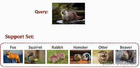
In the image above, let's assume we have a trained image classifier, but the model has never seen an otter. During testing, we want the model to distinguish otters. To achieve this, we provide the model with a Support Set and let it choose which category the query image belongs to within the Support Set.
Few-shot Learning is a type of Meta Learning, which is essentially learning how to learn.
k-way n-shot support Set:The Support Set is a small sample dataset that helps the model distinguish new categories. $k$ represents the number of categories in the small sample, and $n$ represents how many samples there are per category. For example, if there are 3 categories, each with one sample, it is a 3-way one-shot setup.
- k-way: The more categories (k), the lower the classification accuracy.
- n-shot: The more samples per category (n), the higher the classification accuracy.
Basic Idea of Few-shot Learning:The idea is to learn a similarity function $\text{sim}(x, x')$ to determine the similarity between samples $x$ and $x'$. The higher the similarity, the more likely the two samples belong to the same category. For example, we can learn this similarity function from a large dataset and then use it for predictions.
Here, the similarity function refers to the entire model.
Siamese Network
A Siamese Network is a type of network used for few-shot learning.
The training dataset used by this network consists of two parts::
- Positive Samples: Pairs of "same-class" samples $(x_i, x_j, 1)$, where 1 indicates that $x_i$ and $x_j$ belong to the same class. For example: $(\text{Tiger}_a, \text{Tiger}_a, 1)$.
- Negative Samples: Pairs of "different-class" samples $(x_i, x_j, 0)$, where 0 indicates that $x_i$ and $x_j$ do not belong to the same class. For example: $(\text{Car}_a, \text{Elephant}_a, 0)$.
Siamese Network Architecture:
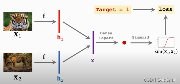
- Model $f$: This can be a CNN (Convolutional Neural Network). Note: The two $f$ networks are the same.
- Vectors $h_1, h_2$: Output vectors of network $f$.
- Vector $z$: A processed version of $h_1$ and $h_2$, for example, $z=|h_1-h_2|$.
- 向量 $z$:对 $h_1$ 和 $h_2$ 进行处理,例如,令 $z=|h_1-h_2|$
- Dense Layers: Fully connected layers.
- ●:The scalar output from the fully connected layer.
The forward propagation of the network:
- Feed two images $x_1$ and $x_2$ into the same convolutional neural network $f$, obtaining output vectors $h_1$ and $h_2$.
- Compute the absolute difference between $h_1$ and $h_2$, resulting in vector $z$.
- Pass vector $z$ through a fully connected network to obtain a scalar.
- Feed the scalar into a Sigmoid function to obtain the final output, which represents the similarity between the two images.
The process for negative samples is the same.
Advanced Architecture: Triplet Loss
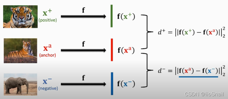
- From the training set, select an anchor sample $x^a$, then choose a positive sample $x^+$ and a negative sample $x^-$ based on the anchor.
- Feed the three samples into the "same" convolutional neural network $f$, and calculate the distance $d^+$ between the positive sample and the anchor, and the distance $d^-$ between the negative sample and the anchor. These distances are calculated as: $d^{+}=\left\|\mathbf{f}\left(\mathbf{x}^{+}\right)-\mathbf{f}\left(\mathbf{x}^{\mathrm{a}}\right)\right\|_{2}^{2}$ , $d^{-}=|| \mathbf{f}\left(\mathrm{x}^{\mathrm{a}}\right)-\mathbf{f}\left(\mathrm{x}^{-}\right)||_{2}^{2}$. Here, $|_2^2$ denotes the squared L2 norm.
- Clearly, we want $d^+$ to be as small as possible and $d^-$ to be as large as possible. This can be visualized as:
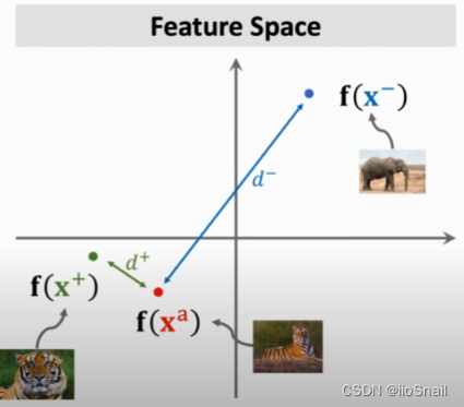
- The loss function is defined as: $$\begin{aligned}Loss(x^a, x^+, x^-)= max\{0, d^+ +\alpha -d^-\}\end{aligned}$$ . where $\alpha$ is a hyperparameter greater than 0. Its meaning is as follows: ① If the distance from the negative sample to the anchor is greater than the distance from the positive sample to the anchor by more than $\alpha$, we consider the pair to be correctly classified, and the loss function becomes 0; ② Otherwise, the loss function is given by $d^+ + \alpha - d^-$.
Pretraining and Fine Tuning
Another approach to Few-shot Learning: Using pre-trained models to perform Few-shot Learning.
Pretrained CNN Models: Use a pre-trained CNN model, and remove the final fully connected layer. The remaining convolutional layers are responsible for extracting features from images, essentially encoding (embedding) the image.
Steps:
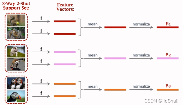
- Use the pretrained model $f$ to extract features from all the small samples, obtaining their feature vectors.
- Combine feature vectors from the same class (in the image above, the average is used), then normalize them. The final result is a vector $u_i$ for each class.
- Once this preparation is complete, you can begin making predictions.
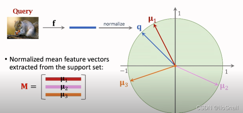
- Extract the feature vector $q$ for the image to be predicted (query image) using the same process as steps 1 and 2.
- Compare the vector $q$ with the class vectors $u_i$. The image belongs to the class whose vector $u_i$ is closest to $q$.
The mathematical formula for this process is:
$$ \begin{aligned} \textbf{p} = \text{Softmax}(Mq) = \text{Softmax}( \begin{bmatrix} u^T_1q \\ u^T_2q\\ u^T_3q\\ \end{bmatrix}) \end{aligned} $$
Simply choose the class with the highest value in $\textbf{p}$.
How to Perform Fine Tuning? The method above only uses the pretrained model without fine-tuning it. Some studies suggest that fine-tuning a pretrained model can improve performance.
Fine Tuning Approach:Replace the fully connected layer of the pretrained CNN with your own, and then train only the fully connected layer using the support set. This can be expressed mathematically as:
$$ \begin{aligned} p_j = \text{Softmax}(W \cdot f(x_j) + b) \end{aligned} $$
Where $f$ is the pretrained model without the fully connected layer, and $W$ and $b$ are the weights and biases for your own fully connected layer. The loss function is simply CrossEntropy.
In fact, the version without fine-tuning above is equivalent to fixing $W$ as $M$ and $b$ as 0.
Fine-Tuning Tips:
- Initializing $W$ with $M$ and $b$ with 0 can yield better results.
- Using regularization in the loss function improves performance.
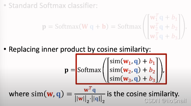
- Modify $Wq$ as follows: change $wq$ to sim(wq). This is said to significantly boost accuracy. See the image below:
Common Few-shot Datasets
- Omniglot:Handwritten alphabet recognition, suitable for academic use. It's only a few MB in size with over 1,600 classes, but each class has very few samples.
- Mini-ImageNet: Image recognition, with 100 classes, each containing 600 samples.
Reference
- https://www.youtube.com/watch?v=UkQ2FVpDxHg


