PyTorch Beginner's Tutorial (6) - Using GAN to Generate Simple Anime Character Avatar
Overview
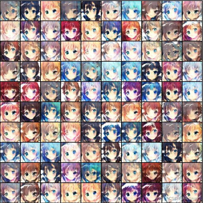
This post is inspired by GAN Assignment 06 from 2021 by Professor Li Yanhong (GitHub link here). The goal is to train a GAN network that generates anime character faces. This is a beginner-level guide, so we’re using the most basic GAN model, which results in somewhat blurry anime faces. After training for just 40 epochs, the generated results look like this:
Global Parameters
First, let's import the necessary packages:
```python
import os
import sys

import torch
import torch.nn as nn
import torchvision
import torchvision.transforms as transforms
from torch.autograd import Variable
from torch.utils.data import Dataset, DataLoader
import matplotlib.pyplot as plt
from tqdm import tqdm
from torch.utils.tensorboard import SummaryWriter
```
Then, set some global parameters:
```python
batch_size = 64
num_workers = 2
n_epoch = 100
z_dim = 100 # Dimension of the noise vector
learning_rate = 3e-4
device = 'cuda' if torch.cuda.is_available() else 'cpu'

# Model save path: if mounted on Google Drive (in Google Colab), the model will be saved there
ckpt_dir = 'drive/MyDrive/models'
faces_path = "faces"  # Directory for the dataset

print("Device: ", device) # Display the device to ensure training is on GPU, not CPU
```
```
Device:  cuda
```
Dataset
The dataset consists of a collection of anime character portraits. You can download it using the following link:
```
https://pan.baidu.com/s/1zsJJJapFLr1zWWhgGol-aA 提取码:2k4z
```
After downloading, extract the contents to the current directory so that the final structure appears as:
```
faces/
├── 1.jpg
├── 2.jpg
├── 3.jpg
...
```
Utility Function
Here, I’ve defined a utility class to clear outputs during training. This helps keep the output area manageable by preventing excessive clutter.
```python
def clear_output():
    """
    Clears the output in a Jupyter Notebook.
    """
    os.system('cls' if os.name == 'nt' else 'clear')
    if 'ipykernel' in sys.modules:
        from IPython.display import clear_output as clear
        clear()
```
Data Preprocessing
We’ll define the Dataset class, resizing each portrait image to 64x64 pixels and standardizing the images:
```python
class CrypkoDataset(Dataset):
    def __init__(self, img_path='./faces'):
        self.fnames = [img_path + '/' + img for img in os.listdir(img_path)]

        self.transform = transforms.Compose([
            transforms.ToPILImage(),
            transforms.Resize((64, 64)),
            transforms.ToTensor(),
            # Here, the images are normalized to have a mean of 0.5 and a standard deviation of 0.5,
            # effectively scaling them with (x - 0.5) / 0.5.
            transforms.Normalize(mean=(0.5, 0.5, 0.5), std=(0.5, 0.5, 0.5)),
        ])

        self.num_samples = len(self.fnames)


    def __getitem__(self, idx):
        fname = self.fnames[idx]
        img = torchvision.io.read_image(fname)
        img = self.transform(img)
        return img


    def __len__(self):
        return self.num_samples
```
```python
dataset = CrypkoDataset(faces_path)
dataloader = DataLoader(dataset, batch_size=batch_size, shuffle=True, num_workers=num_workers)
```
Let's run a quick test to check each method:
```python
dataset.__getitem__(0).size(), len(dataset)
```
```
(torch.Size([3, 64, 64]), 71314)
```
As we can see, the images are successfully resized to 64x64 pixels, with a total of 71,314 images.
Now, let's display a few images to see the results:
```python
images = [(dataset[i] + 1) / 2 for i in range(16)]  # Select 16 images
grid_img = torchvision.utils.make_grid(images, nrow=4)  # Arrange them into a 4x4 grid
plt.figure(figsize=(6, 6))
plt.imshow(grid_img.permute(1, 2, 0))  # plt expects channels at the end, so we use permute
plt.show()
```
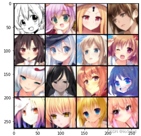
A brief explanation of
(dataset[i] + 1) / 2: Since we previously applied normalization, wherey = (x - 0.5) / 0.5, this line reverses it to retrieve the originalxvalues by applyingx = 0.5y + 0.5 = (y + 1) / 2.
Model Definition
With the dataset ready, we can define our model. A GAN requires both a Generator and a Discriminator. The Generator is responsible for creating images, while the Discriminator evaluates whether the images are generated or real. Here, we use a DCGAN (Deep Convolutional GAN) for this purpose.
Generator
```python
class Generator(nn.Module):
    """
    Input Shape: (N, in_dim), where N is the batch size, and in_dim is the dimension of the random vector.
    Output Shape: (N, 3, 64, 64), generating N color images of size 64x64.
    """

    def __init__(self, in_dim, dim=64):
        super(Generator, self).__init__()

        def dconv_bn_relu(in_dim, out_dim):
            return nn.Sequential(
                nn.ConvTranspose2d(in_dim, out_dim, 5, 2,
                                   padding=2, output_padding=1, bias=False),
                nn.BatchNorm2d(out_dim),
                nn.ReLU()
            )

        # 1. First, use a linear layer to reshape the random vector into a 4x4 image with dim*8 channels.
        self.l1 = nn.Sequential(
            nn.Linear(in_dim, dim * 8 * 4 * 4, bias=False),
            nn.BatchNorm1d(dim * 8 * 4 * 4),
            nn.ReLU()
        )

        # 2. Then, apply a series of transposed convolutions to progressively upscale the image.
        # Each layer reduces the number of channels, ultimately producing a 3-channel, 64x64 image.
        self.l2_5 = nn.Sequential(
            dconv_bn_relu(dim * 8, dim * 4),
            dconv_bn_relu(dim * 4, dim * 2),
            dconv_bn_relu(dim * 2, dim),
            nn.ConvTranspose2d(dim, 3, 5, 2, padding=2, output_padding=1),
            nn.Tanh()
        )

    def forward(self, x):
        y = self.l1(x)
        y = y.view(y.size(0), -1, 4, 4)
        y = self.l2_5(y)
        return y
```
Discriminator
```python
class Discriminator(nn.Module):
    """
    Input shape: (N, 3, 64, 64), where N represents the number of 64x64 color images.
    Output shape: (N,), where each value represents the probability that the Discriminator believes
    the corresponding image is real, with values closer to 1 indicating a stronger belief.
    """

    def __init__(self, in_dim=3, dim=64): # Here, in_dim refers to the image channels, so it is set to 3.
        super(Discriminator, self).__init__()

        def conv_bn_lrelu(in_dim, out_dim):
            return nn.Sequential(
                nn.Conv2d(in_dim, out_dim, 5, 2, 2),
                nn.BatchNorm2d(out_dim),
                nn.LeakyReLU(0.2),
            )

        # This sequence of convolutional layers progressively reduces the image down to a single value.
        self.ls = nn.Sequential(
            nn.Conv2d(in_dim, dim, 5, 2, 2),
            nn.LeakyReLU(0.2),
            conv_bn_lrelu(dim, dim * 2),
            conv_bn_lrelu(dim * 2, dim * 4),
            conv_bn_lrelu(dim * 4, dim * 8),
            nn.Conv2d(dim * 8, 1, 4),
            nn.Sigmoid(),
        )

    def forward(self, x):
        y = self.ls(x)
        y = y.view(-1)
        return y
```
```python
G = Generator(in_dim=z_dim)
D = Discriminator()
G = G.to(device)
D = D.to(device)
```
Since the Discriminator is handling a binary classification problem, Binary Cross Entropy is used here.
```python
criterion = nn.BCELoss()
```
```python
opt_D = torch.optim.Adam(D.parameters(), lr=learning_rate)
opt_G = torch.optim.Adam(G.parameters(), lr=learning_rate)
```
Training the Model
We’ll use TensorBoard to log the changes in loss and to visualize the generated images:
```python
writer = SummaryWriter()
```
Now you can start TensorBoard with the following command:
```python
tensorboard --logdir runs
```
Begin training:
```python
steps = 0
log_after_step = 50 # Log the loss every 50 steps

# z vector for evaluation phase
z_sample = Variable(torch.randn(100, z_dim)).to(device)

for e, epoch in enumerate(range(n_epoch)):
    total_loss_D = 0
    total_loss_G = 0

    for i, data in enumerate(tqdm(dataloader, desc='Epoch {}: '.format(e))):
        imgs = data
        imgs = imgs.to(device)

        # Recalculate batch_size in case the last batch is smaller
        batch_size = imgs.size(0)

        # ============================================
        #  Train the Discriminator
        # ============================================
        # 1. Generate a batch of random noise vectors z
        z = Variable(torch.randn(batch_size, z_dim)).to(device)
        # 2. Get real images
        r_imgs = Variable(imgs).to(device)
        # 3. Generate fake images using the Generator
        f_imgs = G(z)

        # Create labels: real images are labeled 1, fake images are labeled 0
        r_label = torch.ones((batch_size, )).to(device)
        f_label = torch.zeros((batch_size, )).to(device)

        # Use the Discriminator to classify real and fake images
        r_logit = D(r_imgs.detach())
        f_logit = D(f_imgs.detach())

        # Calculate the Discriminator's loss
        r_loss = criterion(r_logit, r_label)
        f_loss = criterion(f_logit, f_label)
        loss_D = (r_loss + f_loss) / 2
        total_loss_D += loss_D

        # Backpropagate for the Discriminator
        D.zero_grad()
        loss_D.backward()
        opt_D.step()

        # ============================================
        # Train the Generator
        # ============================================
        # 1. Generate N fake images
        z = Variable(torch.randn(batch_size, z_dim)).to(device)
        f_imgs = G(z)

        # 2. Calculate the loss; the Generator wants the fake images to look real, so we use f_logit and r_label
        f_logit = D(f_imgs)

        # 3. Calculate the loss; the Generator wants the fake images to look real, so we use f_logit and r_label
        loss_G = criterion(f_logit, r_label)
        total_loss_G += loss_G

        # Backpropagate for the Generator
        G.zero_grad()
        loss_G.backward()
        opt_G.step()

        steps += 1

        if steps % log_after_step == 0:
            writer.add_scalars("loss", {
                "Loss_D": total_loss_D / log_after_step,
                "Loss_G": total_loss_G / log_after_step
            }, global_step=steps)

    # Clear previous output
    clear_output()

    # After each epoch, generate a sample image to check progress
    G.eval()

    # Generate and de-standardize images, then save them to the logs directory
    f_imgs_sample = (G(z_sample).data + 1) / 2.0
    if not os.path.exists('logs'):
        os.makedirs('logs')
    filename = os.path.join('logs', f'Epoch_{epoch + 1:03d}.jpg')
    # Save the generated images
    torchvision.utils.save_image(f_imgs_sample, filename, nrow=10)
    print(f' | Save some samples to {filename}.')

    # Display the generated images
    grid_img = torchvision.utils.make_grid(f_imgs_sample.cpu(), nrow=10)
    plt.figure(figsize=(10, 10))
    plt.imshow(grid_img.permute(1, 2, 0))
    plt.show()

    # Log the generated images in Tensorboard
    writer.add_image("Generated_Images", grid_img, global_step=steps)

    # Switch the Generator back to training mode
    G.train()

    if not os.path.exists(ckpt_dir):
        os.makedirs(ckpt_dir)
    # Save the model every 5 epochs
    if (e + 1) % 5 == 0 or e == 0:
        # Save the checkpoints.
        torch.save(G.state_dict(), os.path.join(ckpt_dir, 'G_{}.pth'.format(steps)))
        torch.save(D.state_dict(), os.path.join(ckpt_dir, 'D_{}.pth'.format(steps)))
```

I stopped the training after reaching the 40th epoch.
Now, let’s take a look at the Tensorboard panel:
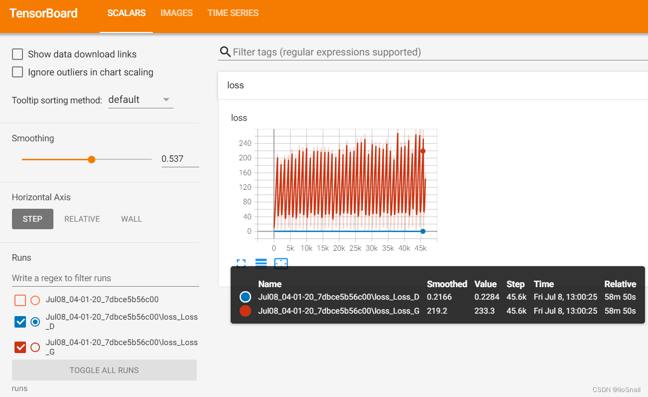
The red line represents the loss of the Generator, while the blue line represents the loss of the Discriminator. From the graph, we can observe two key points:
- The Discriminator's loss is significantly lower than the Generator's loss: This is a common issue with GANs. The Discriminator's task is relatively straightforward compared to that of the Generator—after all, distinguishing between real and fake images is easier than learning to generate convincing images. As a result, the Discriminator might not provide enough useful feedback to the Generator, hindering its ability to converge.
- The Generator’s loss fluctuates continuously (as does the Discriminator’s): Such fluctuations are expected because the Generator's goal is to "trick" the Discriminator. Initially, it fails (higher loss), but then the Generator improves, managing to deceive the Discriminator (lower loss). However, the Discriminator also improves, leading the Generator to fail again, and so the cycle continues. If the Generator’s loss consistently declines, it might indicate that it’s too easy for the Generator to deceive the Discriminator, suggesting that the Discriminator needs improvement.
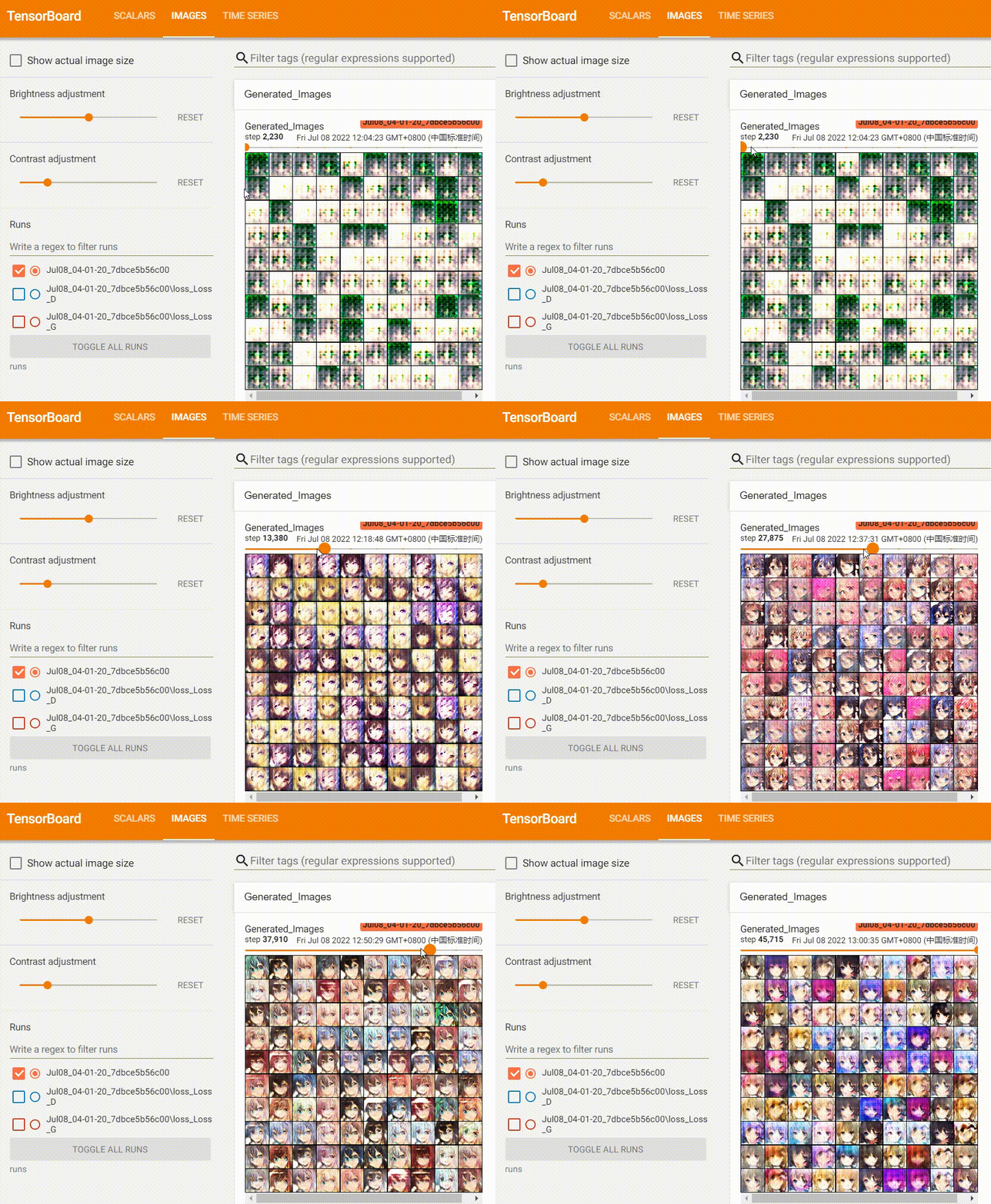
Throughout training, I also documented the progression of the generated images, which show a clear improvement in quality over time.
Using the Model
Once training is complete, let’s test out the model:
```python
G.eval()
inputs = torch.rand(1, 100).to(device)
outputs = G(inputs)
outputs = (outputs.data + 1) / 2.0
plt.figure(figsize=(5, 5))
plt.imshow(outputs[0].cpu().permute(1, 2, 0))
plt.show()
```
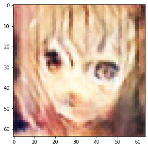
… Well, it’s not perfect, but at least it still resembles a girl!


